We’ve had a number of questions about “measures of dispersion”, such as standard deviation, which tell us how much data spreads out, as opposed to “measures of central tendency”, which tell us where the middle of the data is (as we discussed in Three Kinds of “Average” and Mean, Median, Mode: Which is Best?). Why is the complicated thing called standard deviation preferred over the simpler versions?
Measures of dispersion: Six alternatives
Let’s start in 1996 (anonymous):
Measures of Dispersion

Good day!

I'm from Manila, Philippines. My question is:

What are the different characteristics of these different measures of dispersion:

    a.) Range
    b.) Mean Absolute Deviation
    c.) Standard Deviation
    d.) Variance
    e.) Quantiles (percentile, decile, quartiles)
    f.) CV

I`m not quite sure about that last one's real description... I've gone through different books but still I can't find any answers.

Thanks..:)
All of these are ways to describe the amount of “spread” in a set of data. How do they differ?
Doctor Anthony answered:
Let us go through the list you have given.

(a) Range - Very simple.  This is simply the difference between the largest and smallest members of the population.  So if age is what you are looking at, and the oldest is 90, the youngest 35, then the range is 90 - 35 = 55
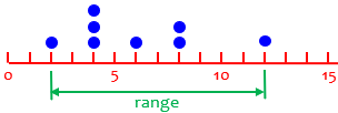
Suppose our data were 2, 4, 4, 4, 6, 8, 8, 12. Then the range would be \(12-2=10\). That tells us literally how far the data are spread out. It depends only on the largest and smallest, so it doesn’t really reflect how all the data are spread.
Here are our data:
This is discussed in detail in Why Are There Different Definitions of Range?
(b) Mean deviation.  First calculate the mean (= total of all the measurements divided by number of measurements)  If the population is made up of x1, x2, x3, ....xn, then mean = (x1+x2+x3+...+xn)/n

If mean = m then to get mean deviation we calculate the numerical value i.e. ignore negative signs of |x1-m|, |x2-m|, |x3-m|, ... |xn-m|  now add all the numbers together (they are all positive) and divide by n.
This is also called the Mean Absolute Deviation, and is the most obvious way to measure how all the data are spread out. For our example, since the mean is \(\frac{2+4+4+4+6+8+8+12}{8}=\frac{48}{8}=6\), the (absolute) deviations are \(4,2,2,2,0,2,2,6\), whose average is \(\frac{4+2+2+2+0+2+2+6}{8}=\frac{20}{8}=2.5\). So on average, the data are 2.5 away from the mean.
For my data above, we have:

If we just added up the signed deviations, \(-4,-2,-2,-2,0,2,2,6\), we would get \(-4+-2+-2+-2+0+2+2+6=0\); this is always true, because in fact the mean is the number that makes the total deviation zero! This is touched upon in Making the Mean More Meaningful.
(c) Standard deviation - This is the square root of the variance, so I will describe that in section (d), and then you get the s.d. by taking the square root of the variance.
This will turn out to be 3, a little more than the MAD.
For my data above, we have:
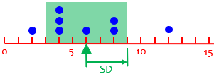
By squaring, we give the greatest deviations a little more influence.
(d) Variance. To avoid the problem of negative numbers we encountered with mean deviation, we could square the deviations and then average those. This is the variance. So variance = {(x1-m)^2 + (x2-m)^2 + (xn-m)^2}/n. As mentioned earlier, the standard deviation is then found by taking the square root of the variance.
Here’s that formula: $$\sigma^2=\frac{\sum_{i=1}^n\left(x_i-\mu\right)^2}{n},$$ where \(\mu\) is the mean.
We’ll see later why this is worth doing. But since squaring distorts values, we take the square root of the mean we get, to clean things up, and get a number with the same units as the data. (The variance itself can’t be shown in a picture!)
(e) Quantiles. You need to plot a cumulative frequency diagram to make use of these. The cumulative frequency shows the total number of the population less than any given value of x. If you plot x horizontally and cumulative frequency on the vertical axis, then to find the median you go half way up the vertical axis, across to the curve and down to the x axis to read off the median value of x. This is the value of x which divides the population exactly in half. i.e. half the population have values below x and half have values above x. The interquartile range is found by going 1/4 and then 3/4 of the way up the vertical axis, across to the curve and down to the x axis. 1/4 of the population have values of x below the lower quartile and 1/4 of the population have values of x above the upper quartile. This means that the middle half of the population have values within the interquartile range. A decile is found by going 10% up the vertical axis, and corresponds to 10% of the population. A percentile represents 1% of the population, so the 30th percentile is the value of x below which 30% of the population lies.
Quantiles (median, quartiles, percentiles) are not in themselves measures of dispersion, but they give a sense of “how far out” a value is relative to everything else, and the IQR (interquartile range) does measure dispersion.
For my data above, we have median (50th percentile) 5, and quartiles 4 and 8 (25th and 75th percentiles, making the IQR 4:
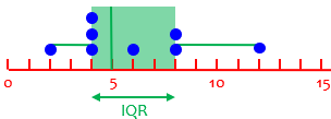
You can see that this is comparable to twice the MAD or SD, but different. It represents the width of the middle half of the data; the drawing here is a essentially box-and-whisker diagram.
The whole concept of quartiles (or quantiles in general) gets complicated, with a variety of definitions. We mention the IQR in Boxes, Whiskers, and Outliers, and in The Many Meanings of “Quartile”, where we see the variations. See also the discussion of cumulative frequency distributions in Cumulative Distribution Functions (Ogive), and in Finding the Median of Grouped Data.
Doctor Anthony misinterpreted the last item in the question, “CV”, as “covariance”, so I’ll omit what he said there; but a year later, reader Amal wrote to correct that:
I _think_ that coefficient of variation might have been what was intended in the question (since everything else was univariate), and that this may also be a more common usage of the abbreviation.

Coeff. of variation is defined as (sd * 100)/mean (see Sokal and Rohlf [1981] _BIOMETRY_, 2nd ed., ch. 4.10).
That is, $$CV=\frac{\sigma}{\mu}\times100\%.$$
We’ll come back to this at the end.
Why use SD rather than MAD? (I)
Next, from 2004:
Why Do We Calculate Standard Deviation the Way We Do?

Why do we square the deviations and then take the square root when calculating standard deviation?  Why can't we just take the absolute value of the deviations?  I've tried similar calculations, and the answers are close, but in most cases, squaring appears to be more correct.
Ah – but how do you define “correct”?
Doctor George gave a quick answer:
Hi Greg,

Thanks for writing to Doctor Math.

There is more than one way to measure the spread of a distribution. Having different methods is a separate issue from the issue of accuracy.  Taking the sum of absolute deviations is a perfectly valid method, but it will in general lead to a different result from standard deviation.  The two methods characterize the spread of the distribution in different ways.

I can think of two reasons why the absolute method is not commonly used.

1. When independent random variables are added their variances add.  Remember that variance is the square of the standard deviation.

2. Variance has the property of being differentiable, which becomes helpful in estimation theory.

Absolute deviations do not have these two important properties.
What he’s saying is that the variance has nice mathematical properties that make it easy to work with in theory. On the other hand, a case might be made that in fact the MAD has a better meaning. (We often describe the SD, simplistically, as a sort of “average deviation”, just because what it really is is harder to follow; MAD is “more correct” as implementation of that intuitive concept.) In particular, the squaring for SD means that greater deviations count for more; data points are treated equally in MAD.
The meaning of the first statement is that if we have two independent quantities (say, measurements of two lengths) that vary with known variances, then their sum will have the sum of those variances: \(\sigma^2(X+Y)=\sigma^2(X)+\sigma^2(Y)\). Its standard deviation, however, will not be the sum of the two standard deviations! Nor is that true for the MAD. And when a mathematician finds something that has a provable quantity, that lets him use it to prove other things – and being able to prove something is like gold to a mathematician!
In particular, with some tweaks we’ll be discussing, the SD of a sample can accurately estimate the SD of the population from which it is taken; this is not true of the MAD.
In addition, the SD works well with the normal distribution, precisely because of its theoretical advantages.
Why use SD rather than MAD? (II)
Back in 1995, we got a two-part question, the first part of which is the same as the last:
Questions About Standard Deviation

Dr. Math,

One of my colleagues here at Friends' Central School in Wynnewood said a question came up in his precalculus class which he could not answer. It's in two parts:

1.  Why does a standard deviation take the square root of the average of the sum of the squared differences between X and X mean instead of the average of the absolute value differences?

2.  What is the reasoning behind dividing by n vs. n-1 in the population versus sample standard deviations?

Well, I couldn't come up with a satisfactory answer, so I'm ASKING DR MATH.
Brad’s second question is largely the topic of next week’s post, so we’ll defer it to then. Here is Doctor Steve’s answer to this first question, offered by a professor (now emeritus) at Swarthmore, where Ask Dr. Math was then based:
Here's a "short" answer from Professor Grinstead. Don't hesitate to write back to have something explained.--Steve

1. The reason that squared values are used is so that the algebra is easier.  For example, the variance (second central moment) is equal to the expected value of the square of the distribution (second non-central moment) minus the square of the mean of the distribution.  This would not be true, in general, if the absolute value definition were used.

This is not to say that the absolute value definition is without merit.  It is quite reasonable for use as a measure of the spread of the distribution.  In fact, I have heard of someone who used it in teaching a course in statistics.  (I think he used it because he thought it was a more 'natural' way to measure the spread.)
The example given is an alternative formula we’ll be seeing next time, which makes the calculation easier: $$\sigma^2=E(x^2)-\left(E(x)\right)^2=\frac{\sum x^2}{n}-\left(\frac{\sum x}{n}\right)^2=\frac{\sum x^2-\frac{1}{n}\left(\sum x\right)^2}{n}.$$
In contrast, absolute values don’t work well with algebra in general; for example, we can expand the square of a difference, \((a-b)^2=a^2-2ab+b^2\), but can’t express the absolute value of a difference, \(|a-b|\) in terms of the absolute values of the individual terms. So the only way to simplify the formula for MAD would be to separate values above and below the mean.
I seem to recall seeing a book that used MAD heavily, as mentioned here, but I can’t find it.
But for now, let’s see how we’ve explained standard deviation itself.
What standard deviation is
Here is a basic question from 1999:
Standard Deviation

What is standard deviation?
Doctor Pat gave a quick introduction:
Rob,

The general idea of a standard deviation is that it is a typical amount to be different. Think of it this way: suppose the average height of 16-year-old males is 70 inches - but almost no one is EXACTLY 70 inches tall. If someone is 71 inches high you will probably still say he is pretty normal in height. Maybe even 72 inches, but at 73 or 74 inches you would start to say that that person is NOT typical; he is on the tall side.

This is sort of what the standard deviation does: it gives us a number to put on sets that says this is (more or less) an unusual measure for this population.
So it gives, in a sense, an average amount of deviation from average; and a deviation greater than that is usually relatively rare. (Note that this oversimplified description, as we’ve mentioned, sounds more like a description of MAD.)
To find it, follow these easy steps:

1) Find the average of the set

2) Create a new set (the deviations) by subtracting the average from each of the original numbers.

3) Square each number in the set of deviations to make a set of squared deviations

4) Average the set of squared deviations

5) Take the square root so that the answer has the same units as the original measures  (ft or inches or whatever)

This is called the root mean square deviation  because it is the ROOT of the MEAN of the SQUARE of the DEVIATIONS.
We’ll see examples and further explanations as we proceed.
A typical example, and a very special case
A question from 1998 asked for more about this (along with an unrelated statistics question I’ll omit):
Standard Deviation and Conditional Probability

Find the standard deviation of the following sample: 5.

My answer is the square root of five. Am I suppose to use some formula?
Read this carefully: the sample Angela is asking about is just the single number 5! It’s not as simple as you might expect.
Doctor Andrewg answered, starting with a more typical example, and explaining the meaning of the whole concept along the way:
Hi Angela!

Okay, first of all let's look at the standard deviation. Standard deviation is a measure of variability in the observations - a higher standard deviation means more variability, and a lower standard deviation means less variability.

Here is a sample with high variability and one with low variability:

     High variability       Low variability
             2                     15
             8                     16
            14                     14
            13                     12
            26                     15
            13                     14
             3                     11

Can you see what I mean? The first column's values are spread out much more than the second's.
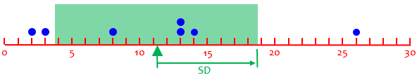
Here is a dot plot of the first dataset:
Here is the second:
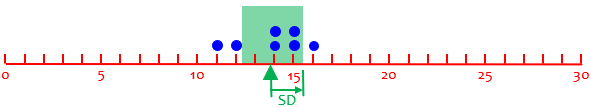
The difference is clear. They have similar means (\(\require{AMSsymbols}{\color{DarkGreen}\blacktriangle}\)), but very different variability. The first will have a greater standard deviation, as shown.
We need a way of quantifying (giving a number that measures) the variability of a sample of observations. This way we can talk about a sample with a standard deviation of 100, say, not just a "large" standard deviation, since in some cases 100 may be a small standard deviation as well, depending on the units we use to measure the observations. Imagine heights measured in meters and then measured in centimeters. Which one looks more variable?
We’ll deal with this issue of units when we get to the coefficient of variation at the end.
For a sample we define the standard deviation as the sum of the squares around the mean, divided by the number of observations. If n is the number of observations, x-bar (the x with a bar over the top) is the mean of the observations, and x_i is the i th observation, then the standard deviation is:

   n
  ---\        _ 2
  \     (x  - x)
  /       i
  ---/
  i=1
  ------------------------
              n
This is the formula we saw before for populations: $$\sigma^2=\frac{\sum_{i=1}^n\left(x_i-\bar{x}\right)^2}{n}$$
You may notice two things here: First, he is using \(\bar{x}\) for the mean, which is traditionally used for the mean of a sample, rather than a population; we haven’t yet made that distinction. Yet he is using \(n\) rather than \(n-1\), which you may be used to for samples. We’ll get into that momentarily.
As an example, here is the calculation for the first example above:
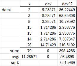
The mean is $$\bar{x}=\frac{\sum x}{n}=\frac{79}{7}=11.29,$$ the variance is $$\sigma^2=\frac{\sum (x-\bar{x})^2}{n}=\frac{395.43}{7}=56.49,$$ and the standard deviation is $$\sigma=\sqrt{\sigma^2}=\sqrt{56.49}=7.52.$$
Now, what about our sample of one?
If you put the single number 5 into that formula, n = 1, x-bar = 5, and x1 = 5. The answer should be zero. This isn't very useful, but it is the only answer I can see here.

So, if 5 is the only number in the sample then the standard deviation for that sample would be zero - there is no variability at all.
Specifically, this is $$\sigma^2=\frac{\sum_{i=1}^1\left(x_i-5\right)^2}{1}=\frac{\left(5-5\right)^2}{1}=\frac{0}{1}=0$$
And this does make sense.
But the way the term “sample standard deviation” is generally used, it means not just the standard deviation of that set, but the adjusted version that estimates the standard deviation of the population, using \(n-1\), as we’ll see next week. And that causes trouble:
If you were using the sample standard deviation to estimate the population standard deviation, then you wouldn't be able to do this with only one observation. The division by n in the formula above would be replaced with a division by (n-1) which is 1-1 = 0 in this case. The standard deviation would then be equal to 0/0 (which is what we call an indeterminate form).
That is, $$\sigma^2=\frac{\sum_{i=1}^1\left(x_i-5\right)^2}{1-1}=\frac{\left(5-5\right)^2}{0}=\frac{0}{0},$$ which can’t be evaluated. Why?
Essentially, a sample of one is all used up in estimating the mean of the population (namely that one value!). So there’s no information left from which to guess how much the population might be spread out. So it should not be surprising that we get an indeterminate value.
What units apply to the standard deviation?
To close, here is a 2003 question with a simple issue:
Standard Deviation and Units

When calculating standard deviation of a data set with units of measure (i.e. centimeters, liters, etc.), is the calculated standard deviation a "unitless" value or does it include units of measure?

For example: would the calculated standard deviation be reported as "0.35" or as "0.35 centimeters?"

It seems to me that standard deviation would be a unitless value, but I repeatedly see people report it followed by inches, gallons or some other unit of measure.
This was briefly touched on above.
Doctor Douglas answered:
Hi, Brandon

The standard deviation has the same units as the original data. For example, you could report the mean and standard deviation of a mass with any of the following:

    102.2 kg +/- 13.6 kg
    102.2 +/- 13.6 kg
    102.2 (13.6) kg

The variance has units of whatever the original data has, but squared (e.g. kg^2 for the above example). There is, however, a quantity that is unitless: the coefficient of variation (CV), which is simply the standard deviation divided by the mean. In the above example, the CV is (13.6 kg)/(102.2 kg) = 0.133.
The standard deviation is measured in the original units. The variance is its square, so it is measured in (typically meaningless) square units. But the coefficient of variation scales this, giving the variation as a multiple of the mean. This way, if we used a different unit, giving larger or smaller numbers, the CV would be unchanged. Think of that 0.133 as saying that the variation is about 13.4% of the mean.
Next time, we’ll explore different formulas, including the sample standard deviation and the alternative formula, both of which we’ve barely touched on.
Pingback: Formulas for Standard Deviation: More Than Just One! – The Math Doctors