(An archive question of the week)
We’ve been looking at some issues involving frequency distributions and the classes used in them. Let’s look at a related concept with some similar issues, namely the cumulative distribution function (CDF), also called an ogive (more on that name at the end of the post!).
What is an ogive?
Here is the question, from 2014:
Ogive, More or Less

I'm doing some exercises on ogive which start with a graph showing information in a cumulative frequency distribution table (also known as cumulative frequency curve). I think I've found an interesting question.

Here's some information about the time it takes 10 runners to complete a track:

         Time    | Upper class boundary | cumulative frequency
  -------------------------------------------------------------
     7-9 seconds |          9.5         |          0
   10-12 seconds |         12.5         |          3
   13-15 seconds |         15.5         |          7
   16-18 seconds |         18.5         |          9
   19-21 seconds |         21.5         |         10

One of my exercises asks me to find x, where 60% of runners took more than x seconds to complete the track.

I reasoned that 60% of 10 runners is 6 runners. And if 6 runners took more than x seconds, that means 10 - 6 = 4 runners took less than x seconds. I didn't draw out the ogive, but let's say from the ogive I found that x is 13.5s.

Now, the interesting question is 13.5s should also mean

   6 runners took 13.5s or more

   AND

   4 runners took 13.5s or less

But the value of 13.5 seconds appears twice, as the boundary for both classes. How weird is that?! How can we say that 4 runners took less than 13.5s but not 13.5s or less?

When we draw out an ogive, the value of any information that we find from the graph seems to have more than one meaning: equal, equal or less than, equal or more than, less than, or more than the value we've found. Is there anyway to differentiate them?

Could you please help? Thanks!
Before we dig into the question itself, let’s pay attention to the terminology, which not everyone will be familiar with.
The word “ogive” (pronounced “oh-jive”), in this context, is another word for a cumulative frequency graph, a visual representation of a cumulative frequency distribution. In this case, we might have started with a frequency distribution like this:
         Time    | frequency
  ---------------------------
     7-9 seconds |      0
   10-12 seconds |      3
   13-15 seconds |      4
   16-18 seconds |      2
   19-21 seconds |      1
This is written in such a way that time is taken as a discrete quantity measured in whole seconds; no runners took less than 10 seconds, 3 took 10, 11, or 12 seconds; and so on. To make the cumulative distribution, we add the frequencies up through a particular class, by adding that class’s frequency to the cumulative frequency before it:
         Time    | frequency | cumulative
  ----------------------------------------
     7-9 seconds |      0    |     0
   10-12 seconds |      3    |     3 (0 + 3)
   13-15 seconds |      4    |     7 (3 + 4)
   16-18 seconds |      2    |     9 (7 + 2)
   19-21 seconds |      1    |    10 (9 + 1)
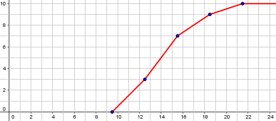
Therefore, the 7, for example, means that 7 runners took anything up through 15 seconds. A graph would look like this, where I am using the class boundaries as Ted did in his question, rather than the class limits as some authors would do):
Ted’s question is about whether the ogive represents the number less than a given value, or less-than-or-equal, and how to handle those boundaries.
Definitions (more or less)
I answered:
There are several things you are missing, all of which are important if you want to fully understand what you are doing.

You say that the meaning of the ogive (CDF) is not clear; but meanings are determined by definitions! What definition have you been given?

Here is one:

  http://en.wikipedia.org/wiki/Cumulative_distribution_function

  The cumulative distribution function of a real-valued
  random variable X is the function given by ...

     F_X(x) = P(X <= x),

  ... where the right-hand side represents the probability
  that the random variable X takes on a value less than or
  equal to x. The probability that X lies in the
  semi-closed interval (a, b], where a < b, is therefore

    P(a < X <= b) = F_X(b) - F_X(a).

  In the definition above, the "less than or equal to"
  sign, "<=", is a convention, not a universally used one
  (e.g., Hungarian literature uses "<"), but is important
  for discrete distributions.

This says that although some sources would use "less than," the standard definition uses "less than or equal." Assuming your class uses the standard definition, there is no ambiguity.
We have seen this several times before, that a convention may not be shared by all mathematicians (not to mention people who merely use math without fully understanding it). In the same way that language varies (I suspect that “ogive” is not nearly as common in the U.S. as in some other countries), definitions themselves can vary.
But we’ll be seeing evidence that Ted’s class does use the “usual” definition.
Boundaries are between values
Second, your example is written assuming that the times are integer numbers of seconds; that is why classes are listed as "7-9," "10-12," and so on, rather than as "7 < x <= 10," "10 < x <= 12," and so on, which would cover all possible values. In this case, you use a class boundary like 9.5 in part to avoid the "or equal" issue: NO value will actually equal the class boundary. So your issue is irrelevant when looking at the actual data. (It would not be irrelevant for other problems involving continuous distributions, but you may not have learned about those yet.)
As I mentioned above, the data are given as a discrete distribution, which is why Ted used boundaries halfway between the limit (e.g. 9.5 between 9 and 10). But this implies that there is no ambiguity in talking about all times less than, or less than or equal to, one of these boundaries, because no time is exactly on one.
What leaves me a little puzzled is that the definition of the CDF fits with continuous classes defined like \(7\lt x \le 10\), but as we’ve seen in recent posts, it is common instead to define them like \(7\le x \lt 10\). I find that to be true among the pages I’ve looked at in writing this post to confirm common usage of the CDF. (On the other hand, several pages I’ve looked at about the ogive, specifically, have used \(7\lt x \le 10\). I’ll look into this below.)
Only an approximation
Third, when you write "60% of runners took more than x seconds," and then attempt to find x, you are actually asking for an approximation, not an exact value. This is because a grouped distribution IS an approximation (ignoring individual values), so that the ogive you draw for this problem is composed of line segments that assume the actual data are uniformly distributed within each class.
In fact, many of the sources I find for drawing an ogive specifically mention that the curve is to be “hand-drawn” (not perfect straight lines), suggesting that the point of the graph is to indicate (subjectively) what the CDF might look like if we used the original data rather than the classes. That is necessarily approximate.
So concern about precision is misplaced; being off by one would not really matter.
Interpreting the intersection
I haven’t really answered his question yet. It will help to make things more concrete:
Let's actually draw the ogive, and consider what it shows us.

I'll assume you have been taught to draw the ogive like this, joining given points by straight lines:

   1.0+                          *
      |                    *
      |                 /
      |              *
      |            /
   0.5+           /
      |........./...................
      |        *
      |      /
      |    /
     0+--*-----+-----+-----+-----+--
        9.5  12.5  15.5  18.5  21.5

There is a straight line from (12.5, 0.3) to (15.5, 0.7). You are looking for the point at which this line crosses the horizontal line y = 0.4 (since if 60% took MORE than x seconds, then 40% took LESS THAN OR EQUAL TO x seconds). Algebraically, you can find that x = 13.25. (If you just drew a graph and measured it, you wouldn't be quite so precise, and your 13.5 may be reasonable.)
This is the graph I drew more exactly above, but this time as a probability distribution, with the vertical axis marked as percentages. Here is my graph with that 40% line added in:
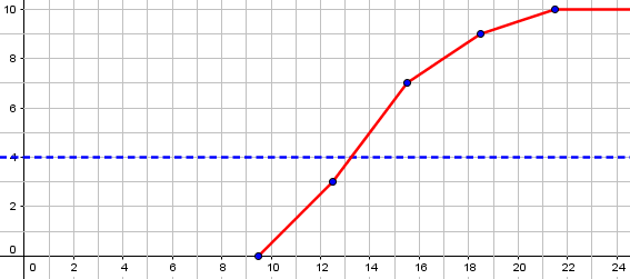
Note also that I quietly corrected a little mistake Ted had made. He said, “if 6 runners took more than x seconds, that means 10 – 6 = 4 runners took less than x seconds.” The last phrase should have been “took less than or equal to x seconds,” which is the proper negation.
Incidentally, what we’ve done here is essentially what I discussed in Finding the Median of Grouped Data.
Now we use the careful definition we had found to interpret what this intersection means, using the points I made earlier:
So the ogive says that

  P(x <= 13.25) = 0.4

The answer is "about 13.25 seconds."

What this means is that about 4 runners took less than or equal to 13.25 seconds, and about 6 took more than 13.25 seconds. It doesn't matter much, though, whether we say "or equal," because (a) the times were measured only to the nearest second anyway; and (b) we don't know the actual times of the 4 who took between 12.5 and 15.5 seconds -- so any answer we give is a guess. It's entirely possible that all 4 had times of 15 seconds, and none took 13 or 14, so that in fact 3 had times less than or equal to 13.25, and there is NO time that EXACTLY 4 of the 10 runners took no more than. This is why I say that anything you determine from an ogive of a discrete distribution will be an approximation, based on a guess about the actual distribution of individuals. Therefore, your concern about "or equal" is swallowed up in bigger inaccuracies.
This is a point I’ve made repeatedly recently: grouping loses information, so everything we say is based on a series of guesses.
The actual cumulative distribution, looking at individuals rather than classes, would not consist of straight lines, or of a smooth curve, but of steps. This is illustrated in the second picture on the Wikipedia page. What you draw is just an approximation of that (and is far more reasonable when the number of individuals is bigger than 10).
Here is the picture I referred to (unless it’s changed since that time):
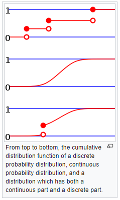 An ungrouped discrete distribution would be like the top graph, with each individual point causing a jump in the cumulative count. But we don’t have that much information.
Your question turns out to be a very interesting one that reveals a lot of facts worth knowing. But did you notice that the question was worded to fit perfectly with the definition of the ogive? It asked about runners taking MORE than a given time, which is the complement of taking LESS THAN OR EQUAL TO that time -- and that is what the ogive explicitly tells you. So if we didn't have all these issues of accuracy, the ogive would give exactly the answer you need.
This is the evidence I mentioned, that this class is using our “less-than-or-equal” definition for the CDF.
Ted responded in a gratifying way:
A good teacher teaches, whereas a great teacher inspires; and Dr. Math, you have inspired me to learn more.

Specifically, I'm going to learn about discrete and continuous probability distributions very soon. :>

But I've learnt a lot already. Thanks!
Further thoughts on continuous classes
I mentioned variations in how classes are defined, with some sources using the (a, b] style that fits with the usual definition of the CDF, and others using the [a, b) style (e.g. by writing “20 – under 30” or \(20\le x \lt 30\)). Here is an example of another question we got (unarchived) about the CDF from 2017:
Does the cumulative frequency (less than type) corresponding to a data value, include the frequency of that data value and the frequencies of all the values less than it, OR does it include the frequencies of values 'strictly less than' it?

What I know is, in case of continuous data type, the value of the Upper Class Boundary (UCB) of a class is not included in that class (it is included in the next class), so the cumulative frequency corresponding to the UCB does not include the frequency of the UCB, it includes frequencies of values 'strictly less than' the UCB.

In case of discrete data type, say for a simple frequency distribution, the cumulative frequency of the first data value is its absolute frequency i.e., in this case the cumulative frequency is not 'strictly less than', it is 'less than or equal to' type i.e. it includes the frequency of the concerned value.

So, my question is, is the definition of cumulative frequency different for different types of data values? Is it 'less than or equal to' for discrete data types and 'strictly less than' for continuous data types? Or, am I wrong somewhere? Also, is the 'greater than' cumulative frequency 'greater than or equal to' or 'strictly greater than'?
Note that Sam’s source used the [a, b) style for classes. Also, the CDF is called “the less-than type” as opposed to the “greater than type”; it is not, apparently meant to exclude “or equal”.
In reply, I referred to the answer above, and added:
Looking around to see what others do, I see some who call it "the less than type", but define it as less-than-or-equal, so the name is not the definition.

But if you use class boundaries rather than limits for a discrete distribution, it won't matter, since the boundaries lie between data values, and won't be hit anyway. (That's part of the reason we define class boundaries that way.) If you go by class limits, then being inclusive makes the result equivalent to using the boundaries. And it really makes no sense to use strict inequality in this case; the Wikipedia quote in the page above seems to agree.

For a continuous distribution, it doesn't really matter which way you define it (in theory) because any one value has zero probability of being exactly one of the data values.

So I think you should always use the "or-equal" definition, unless you are working from a text that says otherwise.
So, for discrete distributions, we take the boundaries between values, so the highest actual value in a class will be included in the cumulative count; for continuous distributions, any one value in principle has probability zero of occurring, so including it or not theoretically should mean nothing. (This is true, for example, of the normal distribution.) But it is entirely possible that a textbook that excludes the upper boundary from a class, would also exclude it from the cumulative count. It would be interesting to do a survey of books and other authorities to see how these choices are correlated.
One more little issue …
Why is it called an ogive, anyway?
As I’ve said, “ogive” is not the term I learned for this kind of curve; but I was familiar with the word before I’d ever seen it in this context. If you are curious, here is a question from 2002:
Origin of Ogive

What is the origin of the term "ogive"? I know what the word means, but I would like to know where the name came from.
Doctor Pat answered:
Part of what is in Math Words and Some Other Words of Interest, at

   http://www.geocities.com/poetsoutback/etyindex.html

under the term ogive is:

"The term was applied by Francis Galton to the cumulative normal distribution but is used more generally now. The word originally comes from a term in architecture for a diagonal rib of a Gothic vault or a pointed arch. The term comes from the Late Latin obvita, the feminine past participle of obvire, to resist."
(The link, to “Doctor Pat” Ballew’s own page of math etymology, is broken, and I can’t find the site’s current location, even through the author’s blog. The origin of the word is not entirely certain.)
Here are some architectural ogive arches:

My impression is that the statistical term relates more to the related concept of ogee arch,

or ogee molding,
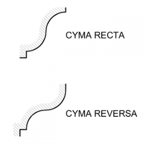
each of which relates to the typical shape of an ogive graph, particularly in the orientation shown as “cyma recta”. The words are closely related, and have been used somewhat interchangeably.
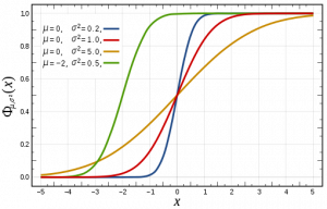
For comparison, here is the CDF of the normal distribution (the red curve is the standard normal):