Bounds on Zeros of a Polynomial

(An archive question of the week)

There are several ways to restrict the range of values you need to test when you are searching for zeros of a polynomial (using the Rational Zero Test or the Intermediate Value Theorem, for example). One of them can be quite useful for difficult problems, but can be hard to follow, and easy to misinterpret.

Upper and lower bound theorems

This 2017 question came from Michael, who was using the Rational Zeros Theorem to try to factor \(x^3 – 4x^2 + x + 6\):

Bound to Confuse

I was able to correctly factor the function below, and others in the textbook, but need some guidance on applying the upper bound theorem and lower bound theorem. I thought they would be very useful as I factor polynomials, but am finding them of limited utility. Either I don't fully understand how to use them as tools, or they are of limited utility, or both.

After you determine a factor and rewrite a function as a product of quotient and divisor, does the theorem apply as you factor the quotient? For example, after dividing the quotient by a divisor you wish to try as a factor, you have all positives in the bottom row of synthetic division table. If your divisor for the quotient was (x - c), is "c" an upper bound for the original function, or only an upper bound for the quotient if it were to be written as a function itself?

If the graph of a function shows a value "c" of the function to be the upper boundary, shouldn't the terms in the quotient for the (x - c) factor be all positive? It doesn't work out that way when I factor P(x) = x^3 - 4x^2 + x + 6 using (x - 3). I get 1 -1 -2 0 in last row of my synthetic division table. 3 is the upper boundary in the graph of the function. (I've had similar experiences on the lower bound side in other problems I've done, i.e., not getting terms that alternate between non-positive and non-negative in the last row).

Again, I can factor the functions, but don't know how best to apply these theorems as tools.

Michael has graphed the function, and observed that the largest zero is x = 3, and the smallest is x = -1.

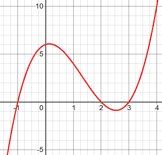
Therefore, 3 is an upper bound of the set of zeros, and -1 is a lower bound. But he finds that the theorem he was taught doesn’t tell him that.

If you are not familiar with the Rational Zeros [or Root] Theorem, see

Rational Root Theorem

I responded:

I think the main issue here is that you are misunderstanding the meaning of "bound," which ought to be clearly stated by any textbook that teaches this theorem, but probably isn't. (My search for information on the theorem showed that you are not alone.) Once you understand the theorem, you will see that it does at least work, which apparently is the main thing you mean by "limited utility."

It happens that it isn't extremely useful (the other aspect of the word "utility") in that you can survive just fine without it. All it does is let you know when you can stop testing possible zeros, if you don't have a graph to go by (which would tell you to stop sooner in many cases). In my school, we don't include the theorem as a course objective, so I don't bother to teach it -- and students do fine! I just tell them that if they read the textbook, it will give them a couple extra tricks they might find useful, but that they don't need.

Michael had found a seeming conflict between what the graph showed and this test; that’s because the test doesn’t tell you as much as the graph does. We’ll see that below. Further, the test is most useful in the hardest cases – perhaps harder than most exercises you are likely to be given.

So let’s look at the theorem:

To answer your first question, c is an upper bound of the set of zeros of the given function. It has nothing to do with the zeros of the quotient (unless the remainder was zero).

I'd like to see how the theorem was stated in your book. How was the term "upper bound" defined, and what examples were given?

Here is the theorem as one source puts it:

  Definition: An upper bound is a number greater than or
  equal to the greatest real zero.

  Upper Bound Theorem:
  If you divide a polynomial function f(x) by (x - c),
  where c > 0, using synthetic division and this yields
  all non-negative numbers, then c is an upper bound to
  the real roots of the equation f(x) = 0.

  Definition: A lower bound is a number less than or
  equal to the least real zero.

  Lower Bound Theorem:
  If you divide a polynomial function f(x) by (x - c),
  where c < 0, using synthetic division and this yields
  alternating signs, then c is a lower bound to the
  real roots of the equation f(x) = 0.

This PDF (125k) includes another, more formal version on its sixth page:

  Some Polynomial Theorems, by John Kennedy (see #10)

There’s a detail in both versions of the theorem that many students miss:

Note that these theorems are about recognizing a number as AN upper or lower bound, not as THE LEAST upper or GREATEST lower bound. It doesn't give an exact boundary line (the largest zero); just some number beyond it. As long as all the zeros are less than or equal to c, it is an upper bound -- so if the greatest real zero is 3, then 3, 4, 5, 6, and 1000 are all upper bounds!

This addresses your second question: it happens that this test does not find 3 to be an upper bound, but it will find that 4 is an upper bound. It's conceivable that it would not find an upper bound until you got to 1000 (though I doubt that would ever happen in a real problem).

More importantly, the theorem only says that IF you get all positive numbers, THEN c is an upper bound. It does not say that IF c is an upper bound, THEN you will get all positive numbers! So if 3 is an upper bound but does not yield positive numbers, that does not contradict the theorem. What would contradict it would be if division by 3 yielded all positive coefficients, but 4 was a zero.

These are things that a good textbook ought to make clear. I suspect that many may not, because they only teach the use of the theorem in a particular context where these questions won't come up (unless the students are actually thinking...).

Here are the synthetic divisions to test 3 and 4 as upper bounds:

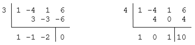
The theorem doesn’t say that 3 is an upper bound (some numbers are negative); it doesn’t claim that it always will! But it does tell us that 4 is an upper bound (no numbers are negative), which is true, though 4 is not the lowest upper bound.

Students at this level don’t have a lot of experience reading theorems carefully. The fact that the theorem only gives “a bound”, not “the best bound” is important, as is the fact that the implication only goes one way.

When is it useful?

Next, I looked at how the theorem is used in practice:

Now let's get to the real question of utility: Who needs this theorem, if it doesn't even claim to find the actual upper bound of zeros?

The place where we use it is in searching for zeros by synthetic division. You typically get a list of possible rational zeros, and test them one at a time. If you have a list of 32 numbers to try, you'd rather not have to  try them all. So you start with the smallest positive number in the list, and work upwards. Each time you find a zero, you replace the original polynomial with the quotient. Each time, you look at the coefficients you got, and if they are all positive, you know that there are no larger zeros, and you can stop. Then you repeat the same process with negative numbers (which you might have been doing in parallel with the positives).

So there's the utility: it allows you to recognize, just by looking at the results of each division you are already doing, when you can stop. Often you will have gone beyond any ACTUAL zeros, and may feel that you have wasted a little effort; but any other method you use to tell when to stop (short of an actual graph) would take more work.

Again, my students don't have any trouble because they were not taught this trick. I tend not to give them problems that have 32 possible rational zeros; and they will have hit all the zeros before they reach the end of the list anyway. You've found the same to be true.

The theorem is perhaps more valuable when there are irrational zeros that have to be approximated, because it helps in locating where they must be. The bounds it gives, even though not as tight as possible, keep you from having to look all the way to infinity. (Of course, if you graph the function, you won't need this.)

The whole point is to save work; and it fits perfectly into this process because you are already doing the divisions anyway – the work is free! In fact, it might be wise to try only integers at first, and then only test fractions that are within the bounds you find.

Michael replied, showing how his book stated the theorem:

My textbook is Stewart, Precalculus Mathematics for Calculus, 5th Ed. It gives the upper and lower bounds theorems as follows:

  Let P be a polynomial with real coefficients.

  If we divide P(x) by x - b (with b > 0) using
  synthetic division, and if the row that contains the
  quotient and remainder has no negative entry, then b
  is an upper bound for the real zeros of P.

  If we divide P(x) by x - a (with a < 0) using
  synthetic division, and if the row that contains the
  quotient and remainder has entries that are
  alternately non-positive and non-negative, then a is
  a lower bound  for the real zeros of P.

After reading your reply, I reread the second example in the book, and I now see that my question about looking for additional zeros when dividing a quotient was answered in the second example in the textbook. I am embarrassed to admit that, but think that it is now unlikely that I shall forget it.

In your reply, you stated that the theorem does not say that if c is an upper bound, then you will get all positive numbers -- that it only says that if you get all positive numbers, then c is an upper bound. Searching for an answer on the web before my original post, I came across a reply that stated that the theorem was a "one-sided logic test," but wasn't entirely certain that I understood that phrase. After reading your more clearly stated response, I now understand what is meant by a one-sided logic test.

I can't thank you enough for the time you gave to address my questions, and for then providing further clarification on the theorem. Math is much more fun when you have a deeper understanding than is necessary to simply solve the problems. There are vignettes in my text on mathematicians, and I am amazed at how long ago some of the principles were discovered....

Refining the method

The textbook is a good one. I replied:

Since this is from Stewart, the theorem is, of course, well stated. I see that the (later) edition I located starts with a nice definition of bounds:

  We say that a is a lower bound and b is an upper bound
  for the zeros of a polynomial if every real zero c of
  the polynomial satisfies a <= c <= b. The next theorem
  helps us to find such bounds for the zeros of a polynomial.

But, typical of the subtlety of reading math, it would be easy to miss the word "such" in that last sentence, and think it said "find THE bounds," rather than what amounts to "find A pair of bounds, which are not necessarily going to be the tightest." Textbook authors aren't able to take as much space as would be needed to prevent all possible misunderstandings, but they do (if they're good) make sure that their few words concisely say exactly what needs to be said, if you read them closely.

The comment about looking for additional zeros brought another issue to mind:

I'm not quite sure how to interpret this comment (I wasn't sure last time either), but if you're saying that you thought that you had to redo the list of possible rational zeros when you have found a zero and move on to use the quotient, then the fact is that *sometimes* doing so *does* help. I hinted at this when I said, "It has nothing to do with the zeros of the quotient (unless the remainder was zero)", referring to the fact that when you do find a zero, the zeros you find for the quotient still have to be in the list you got. I almost said more, but didn't because it wasn't directly relevant to my main point. Now I will.

If the quotient happened to have MORE possible rational zeros than the original, you wouldn't use those, because you already know that they can't be zeros of the original. But sometimes the quotient has FEWER, and then you should remake your list. As an example, suppose (this is part of an example in the edition I looked at) you find that 3/2 is a zero of 2x^4 + 7x^3 - x^2 - 15x - 9, so that you factor it first as (x - 3/2)(2x^3 + 10x^2 + 14x + 6) and then, more usefully, as (2x - 3)(x^3 + 5x^2 + 7x + 3). Now you want to continue; but you notice that the only choices for this are -3, -1, 1, and 3. So you can abandon any other possibilities that were in your original list, knowing that they can no longer work. The book doesn't explicitly point out what is happening here, but does use the conclusion. Perhaps that is what you saw in the example.

This is not about the bounds theorem, but another way to save time in this long, tedious process: Whenever you gain new information, use it!

Michael responded, answering for himself the other interpretation of his question about using the quotient:

In the example in the book, a zero was found for the original function, but it was not an upper bound. When synthetic division was performed on the resulting quotient, a second zero was found, and the third row of entries were all non-negative, so an upper bound was found in this step. The original function was a fifth-degree function. If the quotient were to be viewed as a function unto itself, it would be a fourth-degree function.

I now know that when I have found an upper bound, I have found an upper bound for the original function as well as for the quotient (if considered a function unto itself), because the quotient, as a function unto itself, cannot have boundaries outside those of the original function. I presume that a quotient, when considered as a function unto itself, can have BOTH its upper and lower bounds within the upper and lower bounds of the original function.

In other words, as you use up zeros, you may be narrowing the bounds within which subsequent zeros will be found; but you will never have to widen them, because the quotient has no zeros that are not zeros of the original function.

Then, referring to my point about recalculating the list of potential zeros, he added:

You know, I wish this had been demonstrated in the textbook, but the authors may have considered that the point was intuitively obvious. It did not occur to me until I had done several problems. When I thought of that, I gave myself a "dope slap" for not considering it initially. I guess the optimal situation, as in your example, is when the first term of the quotient is one, and the last term is a prime number.

I closed the discussion with some final comments:

I haven't explored the bounds theorem extensively, so as to be able to say with certainty what things can happen, and what can't. One thing that I have to keep reminding you (and myself) of is that we are not talking about "its upper and lower bounds," but whether any given number is recognized as a bound by the theorem. The actual [tightest or optimal] bounds may not be found by the theorem. Similarly, the theorem can't tell us that a number is not a bound -- only that we don't know it yet.

What we know for sure is that any zero of the quotient will be a zero of the original (since it is a factor of the latter). So even if the theorem could give wider bounds for the quotient than for the original, you would ignore them! Also, any bounds you have found for the zeros of the original will also be bounds for the quotient's zeros. The optimal bounds for the quotient will, as you suggest, be within those of the original, even if we don't find them.

Finally, referring to his comments about things the textbook doesn’t say, I concluded with some words about teaching:

This probably challenges many students. When I teach the material myself, I try to make some of the comments I have been making here; but I doubt that I say everything that could be said, or that it would get through to everyone if I did. Some things can only really be learned by experience, and saying too much only sows more confusion. That's why we give many exercises -- and hope the students actually think while they do them. *Thoughtful* experience is the only way to develop the intuition by which a fact may be "obvious"!
 
It's been interesting digging into this; I'm going to continue thinking about it to develop a better feel for what bounds the theorem does and doesn't find, and whether those bounds always get tighter as you drill down through a sequence of quotients. So thanks for the question!

We can all learn each time we do math.