Last time we looked at some questions about drawing or interpreting the normal curve (graph of the normal distribution). Let’s back up and consider what it actually is. In particular, we’ll see what the “z-score” means.
What is the normal distribution?
First, let’s consider what the normal distribution is, with this question from 2000:
Normal Distribution Curve

Dear Dr. Math,

I am a seventh grader at St. James Middle School, and my question has to do with the normal distribution curve:

When and where did it come into being and what are some of the applications?
Doctor Mitteldorf answered:
Dear Jaime,

A distribution curve is like a histogram where the bars get so close together that each one looks like a line rather than like a bar. You could make a histogram of all the heights of the girls in your class: How many girls are between 4'6" and 4'8", how many between 4'8" and 4'10", etc. If you look at this bar graph when you're done, it will look like a skyline, in which the tallest building is in the middle, and shorter and shorter buildings are around it.
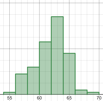
To see how this actually works, I simulated (in Desmos) a class of 100 13-year-old girls (based on the assumption that they are normally distributed with mean 62 inches and standard deviation 2.66 inches, according to American data), Here is a histogram of my sample with 2-inch resolution (the first bar, for example, is 4’6″ to 4’8″):
If we narrow the bars to cover only one inch each, we get this:
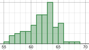
Neither of these looks exactly like the normal curve, which is what we expect in real life.
If you imagine doing the same curve for all the 7th grade girls in the United States, you could make the "width" of each bar much smaller: say, all the girls between 4'6" and 4'6.01", etc. Then you'd have a few thousand different bars, and to plot them all on the same page, you'd have to make each one a thin line. The tops of all the lines together would make a smooth curve, again with the highest point in the middle. This is the distribution curve for heights of 7th grade girls in the country.

In fact, the curve you drew would look approximately like the bell-shaped normal distribution curve that is becoming familiar to you now as you study it. You can take this as an experimental fact about the world. No one can prove it, but it seems to be true that a lot of biological measures like this are approximately normally distributed over a given population.
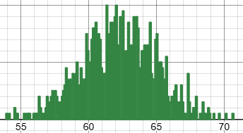
Here is a sample of 1000 girls with 0.1 inch precision:
And here is 10,000 with 0.01 inch precision:
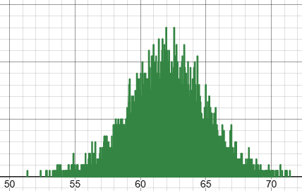
Note that these are not really smooth curves, but rather fuzzy. Yet they are getting closer and closer to that ideal normal curve:
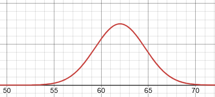
So that’s the idea behind it.
(It would be interesting to find actual data, and see if real girls’ height distribution actually looks like this!)
Why does this happen?
Now, there's a theorem from pure math that hints why the normal curve is so commonly seen in this and other areas. It's not a proof that heights of 7th grade girls are normally distributed - nothing of the sort. It's just an abstract mathematical theorem that seems to have something to do with a lot of real life situations.

The theorem says, roughly, that if you have very many factors contributing to an outcome, and each factor contributes in the same way, then it doesn't matter how the factors are distributed: the net result will be a normal distribution.
That is, because height is determined by a variety of genes and environmental factors, we expect that the distribution would have this form. The theorem is called the Central Limit Theorem.
The actual definition of the distribution was worked out in the 1700’s and 1800’s, based on what we’re about to see: flipping coins.
The classic example of an application of the theorem is this: Experiment A is to flip 4 coins and count how many heads you get. If you repeat Experiment A thousands of times and count how many times you get 0 heads, how many times you get 1 head, etc., and make a bar graph, the bar graph will have a nice symmetric shape, with the highest bar in the middle, at 2 heads. (There are only 5 bars in the bar graph, for 0 heads through 4 heads.)

Experiment B is to flip 100 coins and count how many heads. Now there are 101 possible outcomes, and the bar graph starts to look smoother. Still, there's a tallest bar in the middle at 50 heads, flanked on either side by smaller bars. You can start to see the bell shape in the result. Remember that to collect this data you have to repeat the entire experiment very many times. Each experiment consists of 100 flips, and you have to do the 100 flips thousands of times in order to get a fair sample of the shape of the histogram.

Experiment Z is to flip 100,000 coins. Repeat experiment Z many thousands of times, and make a histogram as you did before. The bars will be very, very close together now. The bars to the left of 48,000 and to the right of 52,000 will be completely empty, because it's so unlikely that you will get a result that departs very much from 50,000 heads. But the area between 48,000 heads and 52,000 heads still has 4,000 bars in the bar graph, and it will look like a very nice outline of the classic normal distribution, or bell-shaped curve.

I don't recommend that you spend your day sitting at home flipping enough coins to do experiment Z. But on a computer, the equivalent experiment is quite feasible, and the programming job should be not too hard for anyone who knows a language like Basic or Pascal or C. LOGO will also work for this.
I used Desmos, which has nice statistical tools. Here is a histogram of the probabilities observed when we flip 4 coins, 10,000 times, together with the corresponding normal curve:
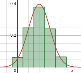
With 10 coins, flipped 10,000 times, we get
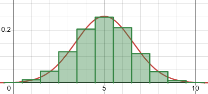
And with 100 coins, flipped 10,000 times, we get
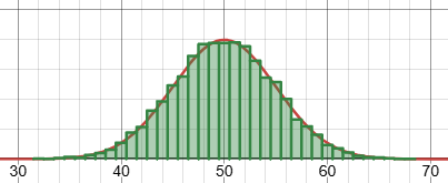
The more coins, the more possibilities, and the closer we get to a smooth curve.
Finding probability in a normal distribution: z-scores
Now that we expect many random variables to have a normal distribution, we want to use that to solve a problem. Here is a question from 2008:
Using Z-Scores to Calculate Probability

Trains carry bauxite ore from a mine in Canada to an aluminum processing plant in northern New York state in hopper cars.  Filling equipment is used to load ore into the hopper cars.  When functioning properly, the actual weights of ore loaded into each car by the filling equipment at the mine are approximately normally distributed with a mean of 70 tons and a standard deviation of 0.9 ton.  If the mean is greater than 70 tons, the loading mechanism is overfilling.

If the filling equipment is functioning properly, what is the probability that the weight of the ore in a randomly selected car will be 70.7 tons or more?
This is a classic type of problem for students just learning about the normal distribution. We’re told that the weights follow an approximately normal distribution (that’s the best we can do in real life!) with specified mean and standard deviation, and are asked to find the probability that the weight in one instance will be in a certain interval. What do we do?
Doctor Grosche answered:
Hi, Kate:

This is a problem in determining the Z-function.  Visualize a diagram of the normal, bell-shaped distribution.  Visualize also how the standard deviation fits in the diagram.  The area under the normal curve from + 1 SD to - 1 SD comprises about 2/3 of the total area of the curve.  That is, for this problem, the mean sits at 70 tons on the horizontal axis and the area under the normal curve from the points on the horizontal axis from 70-0.9 tons to 70+0.9 tons (69.1 tons to 70.9 tons) contains about 2/3 of the area of the whole curve.
We’ll see later what “z-function” (more commonly, z-score) refers to! We’ll also see that his “2/3” is a rough approximation; the probability that a normal variable is within one standard deviation of the mean is actually about 68.26%; many students are taught some approximation of this under the name “empirical rule”.
Here is the graph he has described, showing the area between 69.1 and 70.9:
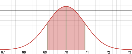
The marked endpoints have z-scores of -1 and 1, meaning they are that many standard deviations away from the mean. Our value of 70.7 in the problem is close to the latter, but not quite, so we’ll have to use something other than memorized numbers.
Now, the area under the curve from - infinity to the mean is half the total area and that from the mean to + infinity is the other half of the total area. In this context area is the same as probability. The question is what the probability is of having 70.7 tons or more of ore in a randomly selected car. Don't let the "randomly selected" bit spook you. That's a necessary precondition for getting a reliable answer. Don't be concerned about how the workers in the field make sure that the car is randomly selected. Just accept, as a given, that they've managed to select the car randomly and go from there.
In real life, you need to be concerned about all these things; but in a textbook problem, you will just assume what they tell you is correct!
Your main task, in a problem like this, is to figure out the critical z-value and to make certain that you pick it correctly.  As you probably know, the formula for z follows:

       x - mu
  Z = --------
        sigma

where x is the point in question, namely 70.7 tons of ore, mu is the mean value (in this case, 70 tons of ore), and sigma is the standard deviation.

      70.7 - 70
  Z = ---------
         0.9

  Z = 0.7/0.9 = 0.778

That gives you the entry-value for the tabulated z-value in your table for the normal curve.  Look at the following link:

  Hyperstat Online: Normal Distribution
    http://davidmlane.com/hyperstat/z_table.html
That page is not a table, as you might expect, but a calculator that does all this work for us, including making the picture.
It's a normal-curve calculator. All you have to do is to put your z-value into the indicated space and it calculates the area or probability for you and gives you a picture of the situation on the normal curve. The only difference from the problem-statement is that the curve is centered on zero as its mean, whereas your problem centers the mean at 70. You can disregard that distinction because calculating the Z-value universalizes the normal curve and centers its mean at zero.
Here is what it looks like when I enter 0.778 as the value above which z has to be:
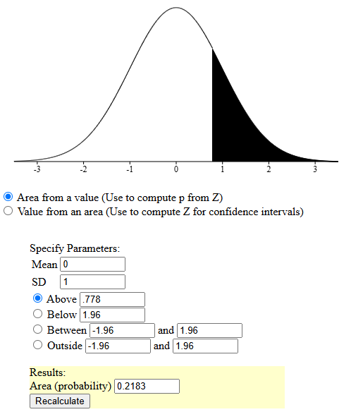
What we have here is called the “standard normal distribution”, with mean 0 and standard deviation 1. The variable z is the input to this distribution.
You are interested in the area of the curve ABOVE the critical Z-value, so put your figure, 0.778, in the indicated space (above) and you see the area or probability: 0.218, to three significant figures, which is usually adequate. The calculator gives you six significant figures but the last three are meaningless, for most purposes.
Actually, that page also allows us to set a specific mean and standard deviation, and directly enter our value 70.7 instead:
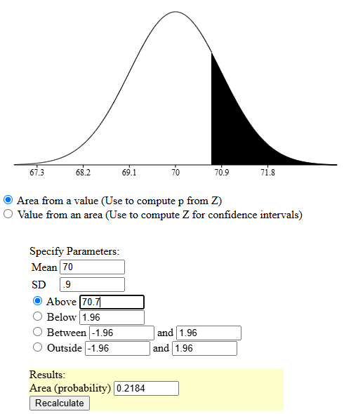
The slight difference in the answer comes from the fact that we rounded z. This time, the page calculated z for itself, internally, with less rounding.
Commonly, in a classroom we would use a table rather than software, though that is gradually changing! Here is an example of such a table:
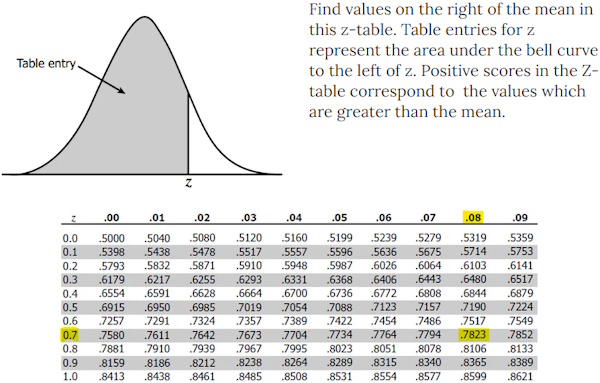
Here I had to round 0.778 to 0.78, because the table only takes two decimal places; and it tells me that the area to the left of this (as shown in the graph) is 0.7823. So the area to the right is 1 minus that, or 0.2177. That would be our (approximate) answer if we had to use this table.
So that’s how we use the z-score to find a probability.
But, what does a z-score mean?
Here’s a question from 2005:
Calculating and Interpreting Z-Scores

Please help me by providing a step-by-step process for calculating the z-score, or standard score.  My class textbook is too confusing.

There seem to be many ways of calculating z-scores, but no standard method that I can apply.  I know how to do standard deviation, but I fall apart when it comes to the z-scores.  Can you help?
Possibly Catherine is referring to different problems in which you can be given different information to obtain z (e.g. from a random variable x, or from a probability). In the absence of an example of her difficulty, perhaps a fresh introduction will help …
Doctor Minter answered:
Hi Catherine!

A z-score is used in statistics to model any normal distribution as a standard normal distribution.  You can consider it "rescaling" the original distribution to fit the properties of a standard normal distribution.  Recall that a standard normal distribution has a mean of 0 and a standard deviation of 1.
We saw this idea above, where the software drew two identical graphs with different scales:
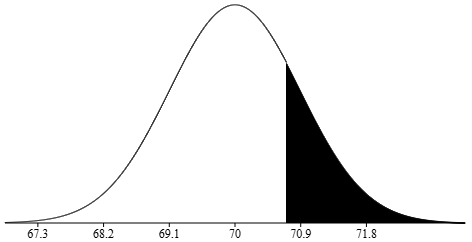
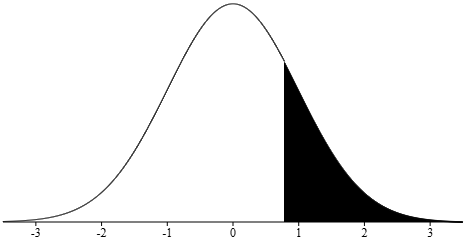
The latter is the standard normal distribution, for which we have tables and simple software; the former is the distribution we are interested in, with numbers taken from a specific problem. By “normalizing”, we make it possible to use known methods for the latter to calculate the former.
If you understand percentages, the concept is very much the same.  If you know what proportion of people in a room have brown hair, say three out of four, you know that 75% of the people in the room have brown hair.

Does that mean that there are exactly 100 people in the room and that exactly 75 of them have brown hair?  That could be the situation, but what if there are only 20 people in the room?

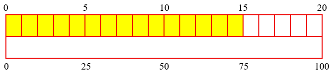
Percentages rescale the actual population.  That is, the percentage tells you how many people in the room WOULD have brown hair if there WERE 100 people, while still having the same proportion as the original group.

A z-score does something not just similar, but EXACTLY like this to a normal distribution to rescale it to a standard normal distribution.  As percentages rescale a proportion to a group of 100, z-scoring rescales any normal distribution to a standard normal distribution.
Here is what that rescaling from 20 people to 100 people looks like:
Let's do an example of a z-score rescaling:

Let's say we have a normal distribution with mean 10 and standard deviation 2.  We'd like to know the probability that a random sampling will produce a value greater than or equal to 11.5.

The standard normal distribution is a bell curve that peaks at zero when graphed, and has a standard deviation of 1.  We need to rescale our distribution do the same.  The z-score conversion formula is

        y - μ
    z = -----
          σ

where y (you might also see it as x, or even another symbol) is our sample value (11.5 in this case), μ (the mean, usually denoted by the Greek letter mu; in this case, μ is 10.), and σ is the standard deviation, usually denoted by the Greek letter sigma, which has a value of 2 in this case.
The numerator finds the distance from the mean to the given value y, and the division finds how many standard deviations that is.
Let's find our z-score:

       11.5 - 10
   z = ---------  = 0.75
           2

So our z-score is 0.75.  What does this tell us?  This value says that if we were to obtain a value greater than or equal to 11.5 by sampling our original distribution, the probability of doing so is the same as the probability of obtaining a value greater than or equal to 0.75 by sampling the standard normal distribution.

If we look at the table for this particular z-score, we see that the probability of a random sampling of the normal distribution yielding a value greater than 0.75, which is equal to the probability of a random sampling of the original distribution yielding a value greater than 11.5, is equal to 0.2266.

That is, 22.66% of random samples from the standard normal distribution will yield values greater than or equal to 0.75, and correspondingly, 22.66% of the random samples of the original distribution will yield values greater than or equal to 11.5.
Here is that work in our table:
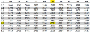
That’s the probability that \(z\le0.75\); the probability that \(z\ge0.75\) is \(1-0.7734=0.2266\).
Here is a graph of our problem,
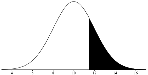
and here is the standardized version:
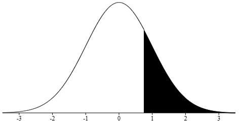
The reason that we do this is because statistics texts have a table of z-scores and their corresponding probabilities.  That handy table of values gives us the probability of z (value obtained by a random sampling of the standard normal distribution) being greater than the z-score obtained by the above formula.  That probability is exactly equal to the probability that the example problem asked us to find!

This process enables us to find the probability that a random sample from ANY normal distribution (there are other distributions also, and this formula does NOT work for them, by the way) is greater than a certain given value.
Our table gives the probability that z is less than a given value, as we’ve seen; and there are others that give the probability that it is between 0 and a given value. See this discussion in Wikipedia, which includes our table (“cumulative”), and one like Doctor Minter’s (“complementary cumulative”), and mentions what I just described, which we’ll see next time (“cumulative from mean”).
If you want to find the probability that a sample produces a value LESS than a certain value, keep in mind that the standard normal distribution is symmetric about zero, and that its total area is 1. You can use these two properties to adjust the process to yield the desired answer. For example, the probability of a random sampling of our original distribution yielding a value less than 11.5 is equal to the probability that we found earlier subtracted from 1, or 0.7734.
Similar adjustments are made for other kinds of tables.
How is that the number of standard deviations?
We’ll close with a 2010 question that went just a bit deeper:
The Idea behind z-scores, and Their Relation to Standard Deviation

I know the definition of a z-score; I know how to compute it, too. But I don't understand why a z-score measures the number of standard deviations an observation is above or below the mean.

What is the concept behind z-scores? What connection do they have to standard deviation?
I answered:
Hi, Charliemagne.

Texts should always explain what I'm about to say, but I get the impression that it's not uncommon to treat z-scores as a bit of magic that you don't need to understand. It's really pretty simple.

The idea is to scale the variable to transform any normal distribution to a STANDARD normal distribution (with mean 0 and standard deviation 1), so that we can just make tables for the latter and not need to handle every possible normal distribution separately.

This scaling involves calling the mean zero, and then measuring the x-axis using the standard deviation as our unit. That is, the z-score is just "how many standard deviations x is away from the mean."
When tables go away and computers do it all, they’ll still use the z-score internally so they only need to program the standard normal. But also, humans will still talk about z-scores in order to compare data informally.
Take an example. Suppose the mean of a normal distribution is 100, and the standard deviation is 15; and suppose our value of x is 130. How many standard deviations from 100 is 130? We first find how far it is:

  130 - 100 = 30

But we want to measure this using the standard deviation, 15. How many 15's are there in 30? We divide 30 by 15 and get the answer, 2. That is, 130 is 2 standard deviations from the mean, 100; so that is what we call the z-score.
The numbers I used are part of the definition of IQ, which is commonly used in examples. So about 2.2% of people can be expected to have an IQ higher than 130. (95.45% are between 70 and 130.)
What we just did was to subtract the mean from x, and divide by the standard deviation:

  x - m
  -----
    s

And that is the definition of the z-score.
That is, $$z=\frac{x-\mu}{\sigma}$$
Another way to see it is to look at a number line labeled with values of x:

  <---+-------+-------+-------+-------+--->
     70      85      100     115     130     x

Subtracting the mean tells how far x is from the mean:

  <---+-------+-------+-------+-------+--->
     -30     -15      0      15      30     x - m

Dividing by the standard deviation tells how many standard deviations x is from the mean:

  <---+-------+-------+-------+-------+--->
     -2      -1       0       1       2     z = (x - m)/s

Since 100 was the mean of x, 0 is the mean of z. And the standard deviation of z is 1. This makes a standard normal distribution, which you can look up in the table.
Next time, we’ll look at a couple more examples, including questions about rounding and other issues.
Pingback: Using a z-Table: Rounding and Interpolating – The Math Doctors