
Last time we looked at the meaning of exponential growth, a term commonly used in describing the initial spread of a virus such as the current SARS2 (which causes COVID-19). But exponential growth can’t continue forever, as it would soon exceed the total population. A slightly more complicated model for growth that takes into account a limited population is called logistic growth; although this is still inadequate to fully predict the growth of a pandemic, it is worth exploring as a simplified model. We’ll look at a few explanations we’ve given for calculus problems about logistic growth, and then compare this with some current graphs that we see, notably the curve we are trying to “flatten”.
One thing we’ll observe is that the equation can be based on quite different parameters, and can be written in significantly different ways, which I hope to untangle.
Infected and uninfected
Our first question is from 2002:
Spread of a Virus Through a City

A Flu-like virus is spreading through a city of population 260,000 at a rate proportional to the product of the number of people already infected and the number of people still uninfected. If 600 people were infected initially and 30,000 people were infected after 10 days, how many people will be infected after 25 days?
The underlying idea here is that, in a limited population (unlike the assumptions for the exponential growth model), not only is the rate of new infections proportional to the number already infected (the more people have it, the faster it spreads), but it must also be proportional to the number available to be infected (the more there are who can get it, the more will). This is still a simplified model compared to real life (where recovery or death removes people from the infected count, for example), but it will be somewhat more realistic. Once the number infected becomes comparable to the total population, that starts to limit growth, and it will no longer look exponential.
Doctor Mitteldorf answered:
Dear Katy,

First, translate the specification in the first sentence into a differential equation.  Then use the second sentence to specify two boundary conditions for the solution.

Let p = 260,000, y = number of people infected, t = time.  Then the first sentence says

   dy/dt = A y(p-y),

where A is a constant to be determined.
You may wonder why it is necessary to define a variable p, when its value is a constant. One reason to do so is to allow us to make a general equation that could be reused for another problem with a different population; another is to avoid having to repeated write a big number (and perhaps make mistakes in doing so).
The derivative can be thought of as the number of new people infected per day; that is assumed to be proportional to the number already infected, and also to the number not yet infected. Now we can solve the differential equation \(\frac{dy}{dt} = Ay(p-y)\), then separating variables to write it as \(\frac{dy}{y(p-y)} = Adt\), and then integrating:
This is called the "logistic equation", and it can be solved by separating variables:

   Integral [dy / (y(p-y))] = At + B,

where B is another constant.

You can do the integral by "partial fractions", noting that

  1/(y(p-y))

can be written as (1/p) (1/y + 1/(p-y))
We commonly call the constant of integration C, but here we have one unknown constant A, and just called the new one B. The method of partial fractions, which we’ll see carried out in another example, transforms the integral \(\int\frac{dy}{y(p-y)}\) to \(\int\frac{1}{p}\left[\frac{1}{y}+\frac{1}{p-y}\right]dy\).
Finish solving the differential equation; then use the second sentence to find A and B. Note that when t=0, y=600; and when t=10, y=30,000.
We’ll be seeing how to finish in the following answers. But for this version, the equation will turn out to be $$y = \frac{p}{1 + ke^{-rt}}$$ where \(k = e^{-Bp}\) and \(r = Ap\) are new constants derived from the arbitrary constants A and B; it doesn’t matter what A and B actually were. Instead, let’s think about what r and k themselves mean.
Observe that as t increases, y approaches p, as expected. (The whole population will eventually be infected in this model, which has no isolation and no immunity.)
The initial number infected (t = 0) is \(\displaystyle p_0 = \frac{p}{1+k}\), so we find that $$k = \frac{p – p_0}{p_0},$$ which in our problem is \(\displaystyle k = \frac{260,000-600}{600} = 432.333\). This is the initial ratio of uninfected to infected.
Similarly, if we know that after T days, the number infected is \(p_T\), then \(\displaystyle p_T = \frac{p}{1 + ke^{-rT}}\); solving this for r, we get $$r = \frac{1}{T}\ln\frac{p-p_T}{kp_T} = \frac{1}{T}\ln\frac{p_T(p-p_0)}{p_0(p-p_T)}$$
In our problem, after 10 days, the number infected is 30,000; so \(\displaystyle r = \frac{1}{10}\ln\frac{30,000(260,000-600)}{600(260,000-30,000)} = 0.40323\).
So the formula for the problem will be \(\displaystyle y(t) = \frac{260,000}{1 + 432.333e^{-0.40323t}}\).
To check, \(\displaystyle y(0) = \frac{260,000}{1 + 432.333e^{0}} = 600\), and \(\displaystyle y(10) = \frac{260,000}{1 + 432.333e^{-0.40323\cdot10}} = 30,000\).
Here is a graph, where the blue curve is our logistic curve, and the red is an exponential with the same rate, obtained by deleting the constant term in the denominator, \(\displaystyle y = \frac{260,000}{432.333e^{-0.40323t}}\):
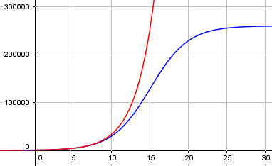
We see that the spread of the virus starts looking exponential, but starts to taper off as an increasing percentage of the population is already infected. We can also see that our r is exactly the exponential rate seen initially; if you have heard \(R_0\) mentioned in discussions of pandemics, this is what that is: the initial exponential rate constant, which is the same idea as the nominal rate in compound interest. The subscript distinguishes it from the actual rate of increase at any point on the curve.
Summarizing, r is a rate constant we can determine from the data; putting in our formula for k, we have the general equation $$y = \frac{p}{1 + \frac{p – p_0}{p_0}e^{-rt}} = \frac{p_0p}{p_0 + (p – p_0)e^{-rt}}$$ where \(p_0\) is the initial infected population and p is the total population. I think this is the most useful form of the equation.
Informed and uninformed
The next question is from 1998:
Logistic Growth of A Rumor Spreading

In a country of 3,000,000 people, the prime minister suffers a heart attack, which the government does not officially publicize. Initially, 50 governmental personnel know of the attack, but spread this information as a rumor. At the end of one week, 500 people know the rumor. Assuming logistic growth, find how many people know the rumor after two weeks.

What I want to know is the basic concept of exponent and some formulas related to this question.
This problem is very much equivalent to the last one, with a known total population and the number “infected” at two different times. It’s just a different “infection” being spread.
Doctor Anthony took this one, taking the same definition of logistic growth but with a slightly different approach:
The logistic differential equation assumes that the rate of spread of a rumor is proportional to the number who know and the number who don't know. If we let x = proportion of the population who know (0 < x < 1), then:

     dx/dt = kx(1 - x)    where k is a constant.

        dx
     --------  = k*dt
     x(1 - x)
This is the same differential equation, except that x is now a proportion (think of it as a percentage), so the total population has been replaced with 1. The actual number of people will be x times the total population. (This is an alternative way to avoid having to keep writing a big number!)
This time, the details of the work for “partial fractions” are shown, solving a system of equations for the two unknown numerators:
Now split up the left hand side using partial fractions:

         1          A        B
     --------   =  ---  +  -----
     x(1 - x)       x      1 - x

Then:

         1          A(1 - x)        B(x)
     --------   =  ----------  +  --------
     x(1 - x)       x(1 - x)      x(1 - x)

So:

     1 =  A(1 - x) + Bx

     1 =  A + x(B - A)

Thus:

      x = 0   1 =  A
      x = 1   1 =  B

                       1            1        1
so we can express  ---------  as   ---  + -------
                    x(1 - x)        x     (1 - x)
The same result was provided for free in the first problem.
So we have:

     INT[1/x + 1/(1 - x)]dx = INT[k*dt]

     ln(x) - ln(1 - x) =  kt + constant

     ln(x/(1 - x)) = kt + constant

     x/(1 - x) = e^(kt+constant)

     x/(1 - x) = Ae^(kt)       where A = constant.
That is, integrating $$\int\left(\frac{1}{x}+\frac{1}{1-x}\right)dx = \int k dt,$$ and exponentiating each side, we get $$\frac{x}{1-x} = Ae^{kt}.$$
Doctor Anthony doesn’t bother to solve for x, but finds the values of constants A and k first, which as we’ll see is very wise:
Then at t = 0:

     x = 50/(3*10^6)    and     1 - x = 1 (approx)

So: 50/(3*10^6) = A

So we get:

     x/(1 - x) = 50/(3*10^6) e^(kt)
Note the approximation he could make because x is very small; our initial proportion is close enough to 0 to ignore in the denominator.
In general, if the initial number “infected” with the rumor is \(N_0\), so that the initial proportion is \(\displaystyle x_0 = \frac{N_0}{P}\), then, setting t = 0 in our general equation, we find that $$A = \frac{x_0}{1 – x_0} = \frac{\frac{N_0}{P}}{1 – \frac{N_0}{P}} = \frac{N_0}{P-N_0}$$ (without approximating).
Now we have a value for A; next we find k:
When t = 1:

     x = 5000/(3*10^6)      and 1 - x is still 1 (approx)
                            actual value is 0.99833

     5000/(3*10^6) = 50/(3*10^6) e^k

     100 = e^k

and so:

     k = ln(100) = 4.60517

Thus our equation becomes:

     x/(1 - x) = 50/(3*10^6) e^(4.605t)
Here, if we know the proportion \(\displaystyle\frac{N_T}{P}\) “infected” at time T, we can solve for k:
$$\frac{\frac{N_T}{P}}{1-\frac{N_T}{P}} = Ae^{kT}\;\Rightarrow\;k = \frac{1}{T}\ln\left(\frac{\frac{N_T}{P}}{A\left(1-\frac{N_T}{P}\right)}\right)\\\Rightarrow\;k = \frac{1}{T}\ln\left(\frac{\frac{N_T}{P}}{\frac{N_0}{P-N_0}\left(1-\frac{N_T}{P}\right)}\right)\;\Rightarrow\;k = \frac{1}{T}\ln\left(\frac{N_T(P-N_0)}{N_0(P-N_T)}\right)$$
Note how useful it was to leave the equation not yet solved for x while finding these constants.
Since the goal is to find one specific value, Doctor Anthony chose just to solve for that value:
Putting t = 2, we get:

     x/(1 - x) =  50/(3*10^6) (10000)

     x/(1 - x) =  500000/(3*10^6)

               =  1/6

            6x = 1 - x

            7x = 1

             x = 1/7

So 1/7 of the population knows the rumor, and 1/7 * 3*10^6 = 428,571 people.

And so after 2 weeks, 428,571 people will know the rumor.
Let’s go back and find the general formula for x: $$\frac{x}{1-x} = Ae^{kt}\;\Rightarrow\;x = Ae^{kt} – x\cdot Ae^{kt}\;\Rightarrow\;x + x\cdot Ae^{kt} = Ae^{kt}\\\Rightarrow\;x = \frac{Ae^{kt}}{1 + Ae^{kt}} = \frac{A}{A + e^{-kt}}$$
To get the actual number N at time t, we multiply this by P: $$N = \frac{AP}{A + e^{-kt}}$$
Inserting our formula for A, we get the same equation we ended up with above: $$N = \frac{N_0P}{N_0 + (P – N_0)e^{-kt}}$$
Birth and death rates
Our last question is from a little earlier in 1998, and is based on very different premises:
The Logistic Model for Population Growth

I have a problem in my high school calculus class. It is known as the Logistic Model of Population Growth and it is:

   1/P dP/dt = B - KP

where B equals the birth rate, and K equals the death rate. Also, there is an initial condition that P(0) = P_0. I need to calculate P(t), which will predict the population at any time. I also need to find the limit of P(t) as t approaches infinity.
This time, we don’t have a population size, and the rate of growth is not based on that, but rather on two (presumably known) rates. Let’s take a moment to ponder what it means, and in what sense B and K can be called birth and death rates.
The left-hand side of the equation as given is the rate of change of population, divided by the population; that is, it is the relative rate of increase. In exponential growth, this would equal a constant: \(\displaystyle\frac{1}{P}\frac{dP}{dt} = B\). B here would be the growth rate; calling it the (initial) birth rate (births per year per animal, say) makes sense. (It’s the \(R_0\) mentioned above.) The model has been modified in the simplest possible way, by reducing the growth rate linearly as the population grows. So K is actually the rate at which the “birth rate” is diminished as population increases.
Doctor Anthony answered this one, this time using the actual population as the variable, rather than a proportion:
We start with the following equation:

   dp/dt = p(b - kp)

Rearranging the equation so that p is on the left and t is on the right, we get:

      dp
   -------- = dt
   p(b - kp)
The same method of solution applies as above, but the partial fractions are a little more complicated:
Use partial fractions for the left hand side:

       1        A       B
   --------- = --- + ------
   p(b - kp)    p    b - kp

   1 = A(b - kp) + Bp

Then:

   p = 0 gives 1 = Ab and so A = 1/b

   p = b/k gives 1 = Bb/k and so B = k/b

The left hand side can then be written:

     1        k
   [--- + ---------] dp = dt
     bp   b(b - kp)
Integrating \(\displaystyle\int\left(\frac{1}{bp} + \frac{k}{b(b-kp)}\right)dp = dt\), we get
   (1/b)[ln(p) - ln(b - kp)] = t + constant

   ln[p/(b - kp)] = bt + constant

   p/(b - kp) = Ae^(bt)            where A is a constant

   p = (b - kp)Ae^(bt)

   p = Abe^(bt) - Akpe^(bt)

   p(1 + Ake^(bt)) = Abe^(bt)

          Abe^(bt)
   p = --------------              (Equation 1)
        1 + Ake^(bt)
This is the same equation we had before, but with different constants: $$p = \frac{Abe^{bt}}{1+Ake^{bt}}$$
We find the constant A from the initial value as before:
At t=0, p = p(0), so we have:

   p(0)/(b - k*p(0)) = A           (Equation 2)

For any given problem, you can calculate A from (2) and then substitute for A in (1).

Dividing (1) top and bottom by e^(bt), we get:

            Ab
   p = ------------
       e^(-bt) + Ak

and as t -> infinity, the term e^(-bt) -> zero, and we have:

                  Ab     b
   p(infinity) = ---- = ---
                  Ak     k
This is the “carrying capacity”, the maximum population that the graph will reach. If we call this C (which plays the role of the total population P in the previous problems), so that \(b = kC\), and replace A with \(\displaystyle\frac{P_0}{b – kP_0} = \frac{P_0}{kC – kP_0} = \frac{P_0}{k(C – P_0)}\), the equation can be written as $$p = \frac{ \frac{P_0}{k(C – P_0)}kC}{ \frac{P_0}{k(C – P_0)}k+e^{-kCt}} = \frac{P_0C}{P_0+(C – P_0)e^{-bt}}$$ This is the same as our previous formulas; the birth rate b plays the role of r, as expected, and the carrying capacity C was calculated as b/k.
The curve we need to flatten for COVID-19
The graphs of total cumulative infections that we most often see, which initially look exponential (see last time), will eventually look more like the logistic curve, as everyone who will be infected becomes infected. If we look at a country that is past its crisis (we hope), we can expect to see something more like the logistic curve. Here is South Korea, from Worldometers:
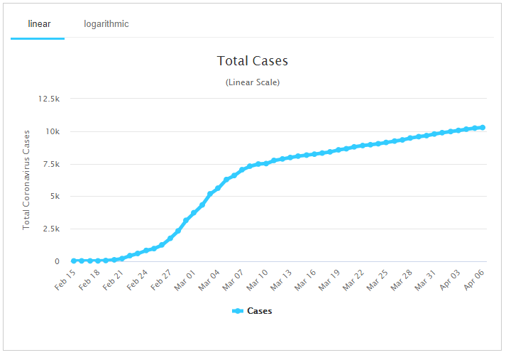
This has changed from an approximately exponential curve at the start to one that looks linear – not finished growing, but manageable. I will make no attempt to explain why it looks this way; that is for the epidemiologists!
For comparison, here is a graph of daily new cases in South Korea, from the same source:
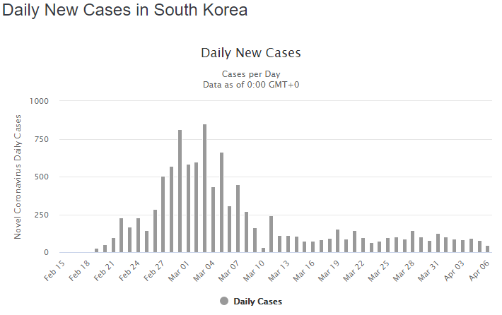
This shows that new cases continue steadily, accounting for the constant upward slope in the first graph.
And that is the curve we are told we want to flatten, as in this graphic from information is beautiful:
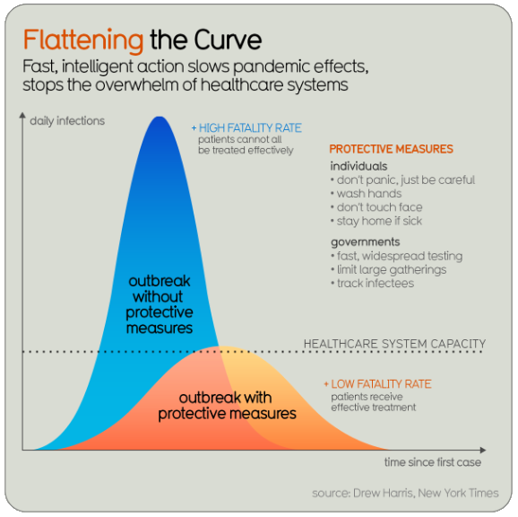
These curves represent the number of daily infections (new cases) – that is, the rate of increase of the cumulative total; in effect, its derivative. The area (integral) under this curve is the cumulative total we have been looking at; the idea is that even if the total number of cases is the same, if we slow down the rate, we can need fewer resources at a given time. Here is an earlier source of this concept, in a paper from 2017 at the CDC:
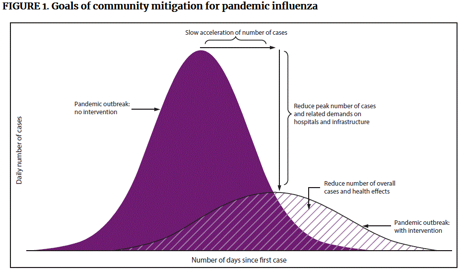
Something I think is commonly misunderstood is that “flattening the curve” refers not to the slope of the cumulative graph finally turning downward, away from the exponential curve, but to making the entire curve lower from the start, something that required effort long before we see a downturn. It means keeping the number of new cases as low as possible.
What happens if we take our logistic curve from the first example above, and graph its derivative (rate of change)? Here it is:
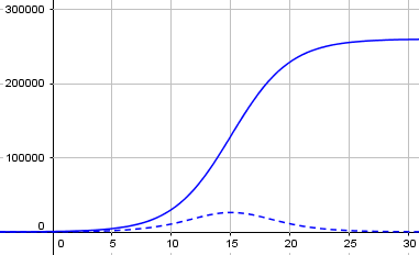
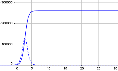
The broken line at the bottom is the rate of change of the growth curve; you can see that it is highest where the growth curve is steepest, at the middle, and symmetrically rises and falls. This is what we want to flatten; and we do that by decreasing the growth rate parameter. Here is what that graph would have been with r = 2 rather than 0.4:
Now, this is a simplified model, as I’ve said all along. I found a nice explanation of what might be called the next step in accurate modeling, the SIR (Susceptible-Infectious-Resolved) model, in a video by Numberphile. Here is my own copy of their GeoGebra graph:
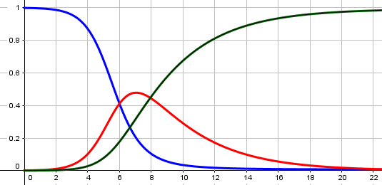
The blue line is the number of people who have not yet been infected (susceptible); the red line is the number who are currently infectious (which is a more accurate version of the curve we want to flatten); and the green line is those who have recovered or died (resolved or removed). Our cumulative total would be the sum of the red and green, and would look like the blue line flipped over. That is virtually identical to the logistic curve.
Next time, I want to look more deeply at something we touched on last time, namely the use of logarithmic graphs to recognize exponential growth.
Pingback: Logarithmic Graphing – The Math Doctors
Pingback: Reading Pandemic Graphs – The Math Doctors