There are a number of standard techniques for graphing functions, such as transforming simple functions, or finding asymptotes and holes for rational functions, and using calculus to find slopes. What if you have a rational function of a trig function, and can’t yet use calculus to figure it out? We’ll look at how we can twist our minds around an unfamiliar function, and we’ll also review the concept of asymptotes.
Sketching a secant
We’re going back to early April for this question:
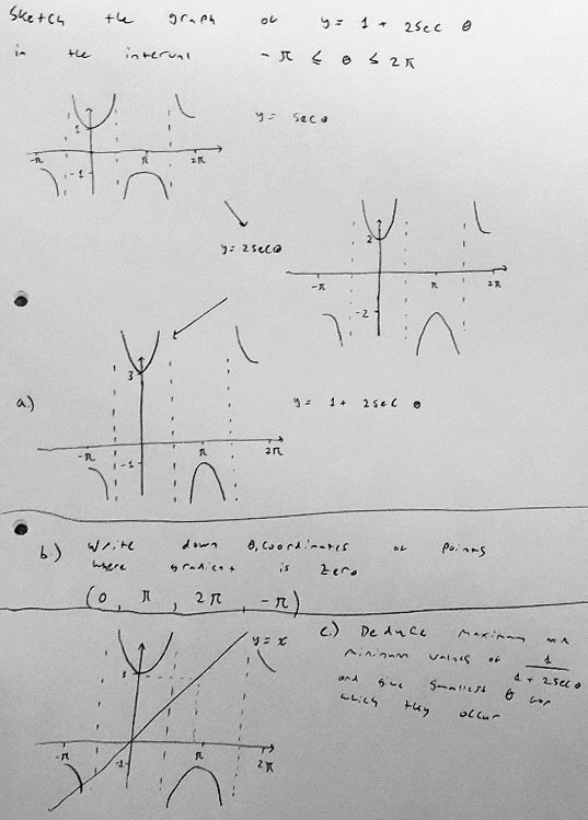
I’m attempting question 10, and I have been able to complete parts a and b, however, I’m stuck on part c.
We’ve not yet covered differentiation of trig functions so I can’t see why that would be part of the question. I thought at first that I needed to sketch the inverse function but I realised that 1/(1+2secθ) is the reciprocal. I can’t figure out where to go from here. Any help is appreciated.
Normally, when you are asked where the gradient (slope) is zero, you find the derivative. Here Frankie is apparently expected to use knowledge of graphs to determine it indirectly.
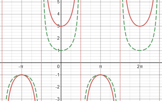
He has correctly graphed \(y=1+2\sec(\theta)\) by a series of transformations from \(y=\sec(\theta)\), and found the points where the graph is horizontal (so the gradient must be zero). Here is an “official” graph showing both functions (secant in green, stretched and shifted up in red, but not strictly restricted to the specified interval):
Now, part (c) is about the reciprocal of this function; a graph is not required, just extrema, based on this graph. At least imagining the reciprocal graph, though, will be useful.
What the reciprocal does
Doctor Fenton answered with a simple hint:
When you have a fraction whose numerator and denominator are both positive, then the fraction gets larger when the denominator gets smaller while the numerator stays the same (or when the numerator gets larger while the denominator stays the same, but that is not the case here). For example, 3/4 > 3/5.
If the fraction has a negative value and the numerator stays the same, then when the denominator gets smaller, the fraction has a larger magnitude (absolute value), but a negative number with a larger magnitude is “smaller” in the sense of being further left on the number line: -3 is to the left of -2, so we write -3 < -2; and 3/(-5) > 3/(-4). You have to use this meaning of smaller when finding maxima and minima of functions. Because of these facts, you don’t need calculus. You can tell just using the graph.
So you have the graph of y=1+2 sec x on the interval [-π,2π]. At what points will the function y=1/(1+2 sec x) have a (local) maximum? Where will it have a local minimum?
So the reciprocal function is increasing where the original is decreasing; and that should mean it will have a maximum where the original has a minimum … but there are some twists involving asymptotes and zeros.
Frankie replied,
Well, I’m not sure where the extrema are located. I was thinking maybe the local maximum could be as x approaches 3pi/2 or pi/2 as 1+2 sec(theta) will get smaller and smaller so the reciprocal will get larger and larger but I don’t know if this is a possible answer since it is undefined at these values so we could not produce any values for them so the local maximum maybe is just at pi. For the local minimum I had the same confusion i.e. that the local minima were at the asymptotes (-pi/2 and pi/2) but again this would mean we couldn’t get a value for 1+sec(theta) and also that pi/2 is related to both the minima and maxima so perhaps it is just at 0 or -pi as these can give a value for 1/(1+2sec(theta)) and have gradients of zero?
There are some good thoughts here, but he’s getting confused trying to think too abstractly.
Graphing to understand
I joined the discussion hoping to help him gain the hands-on experience needed to support such thinking:
Hi, Frankie.
I want to jump in here to suggest something that may help.
Don’t think too much about the specific question yet; you may first have to develop your sense of what taking the reciprocal of the function does, so you can see the implications.
Instead, just take your graph of 1 + 2 sec(θ) and use it to sketch a graph of 1/[1 + 2 sec(θ)] point by point, while thinking about what will happen at other nearby points.
Start with the relative minima and maxima on the graph you made. You have a point (0, 3); on the new graph, there will be a point (0, 1/3). Do the same for other similar points.
Now think about what will happen to points near each of those. Near θ = 0, your graph is higher than 3, so the new graph will be a little lower than 1/3, right? So which direction will the graph curve? Make a little curve showing that.
How about the asymptotes? As θ approaches π/2 from the left, the graph you have rises to +infinity. What will happen on your new graph? What happens on the right?
Show us the graph you make, and tell us what you found as you made it. Then we can talk about the implications for the question you were asked.
The key idea will be to consider the key points on the original graph, and learn to see how the graph will behave near them on the new graph, using Doctor Fenton’s ideas.
What happens to extrema and to asymptotes?
Doctor Fenton first pointed out a possible ambiguity:
You have a correct graph for y = 1 + 2sec x, and it is in four disconnected pieces. Two of them look like a U or an inverted U. Where are the local maxima and minima of these two pieces? The other two pieces each look like half of a U (or inverted U).
The problem just says “extrema” and doesn’t specify whether it means local extrema or absolute extrema. Usually, when we talk about local extreme points, there must be an open interval which contains the extreme point, and that point is larger than all the other points in the open interval (for a local maximum), or smaller that all the other points in the open interval (for a local minimum). An absolute maximum [minimum] is the largest [smallest] value of the function on the entire interval. When you have a graph on a closed interval, as in this case, you need to say whether you can talk about things like derivatives (or gradients) or relative extrema at the endpoint of the interval.
This doesn’t ultimately affect the problem, but it’s a valid concern.
The graph of y = 1 + 2sec x is in four pieces, and the graph of y1 = 1/(1 + 2sec x) will also be in four pieces (although if you graph it, it will look like a single continuous curve). (I’m calling the second graph y1 so we can tell more easily which graph I mean.) It is clear from your graph that when x = 0, y = 3, so y1 = 1/3. If 0 < x < π/2, then y > 3 (so y1 < 1/3, while if -π/2 < x < 0, y > 3 (so y1 < 1/3) also. That means that y has a relative minimum at x = 0. What does y1 have at x = 0?
Here we are thinking about behavior of the new graph at the point corresponding to a relative minimum of the original function. Since the original function is higher on either side of \((0,3)\), the new function must be lower near \((0,\frac{1}{3})\), making that a relative maximum.
Note that y has a vertical asymptote at x = -π/2, and that when x < -π/2, then y < 0, while if
-π/2 < x < 0, then y > 0. What can you say about lim(x→ -π/2–) y1 (the limit from the left)? What about the limit from the right, lim(x→ -π/2+) y1 ?
Where the original graph rises toward infinity, the new graph must fall toward zero.
The graph
Frankie answered, providing a (mostly) reasonable graph:
I have drawn a sketch of the function. As I went along I noticed all points below the x-axis (excluding -1) got larger/closer to positive infinity but smaller in magnitude, and conversely above the x axis all the points got smaller/further from positive infinity, though again all points got smaller in magnitude. This makes sense that all points besides those with a value of 1 would get smaller in magnitude. Also as the values approached the asymptotes of the original graph they all approached zero but would never reach since this would mean the function would be undefined, so there would now be an asymptote at y = 0.
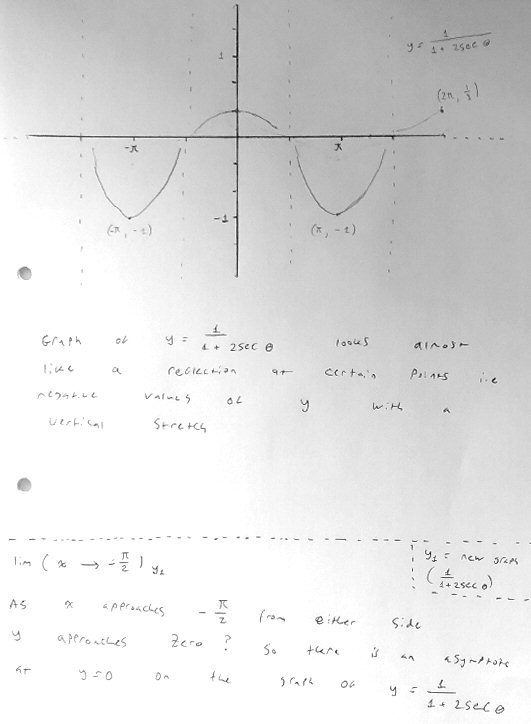
I think the part about magnitudes and infinity was an echo of Doctor Fenton’s statement that “a negative number with a larger magnitude is ‘smaller’ in the sense of being further left on the number line”. The reciprocal of a negative number has smaller magnitude than the number itself, and is therefore greater (“closer to positive infinity”) than the original. A better point would have been that as the negative value of the original function increases toward the relative maximum of -1, its reciprocal decreases toward -1, which will therefore be a minimum.
The point about the new graph approaching zero where the original had an asymptote, is correct. We’ll discuss the wrong claim of an asymptote at \(y=0\).
Back to the point(s)
Unfortunately, where he had previously given correct extrema (though without knowing which were correct), he has been distracted from the goal by my recommendation to graph the function.
Doctor Fenton responded:
You seem to be getting away from the question, which was to find the maximum and minimum values of y = 1/(1 + 2 sec x) on the interval -π ≤ x ≤ 2π.
You are also discussing asymptotes, but there are no vertical asymptotes of y = 1/(1 + 2 sec x) in the interval (there are two points where it is undefined), and you cannot have a horizontal asymptote on a finite interval. Your graph is roughly the right shape, and you should be able to determine the maximum and minimum points on the interval on it.
Frankie replied with the correct answer:
For the extrema I can now see where they are, -1 is the minimum value of the function and this occurs at -pi and pi since the question asks for the smallest positive value this must be pi. As for the maximum this occurs at 0 and 2pi.
I have a question. If the graph did not have a finite interval would there be an asymptote at y = 0? As surely no value could be 0 due to the equation being 1/(1+2 sec(theta)).
The minima are at \(\left(\pi,-1\right)\) and \(\left(-\pi,-1\right)\); the maxima are at \(\left(0,\frac{2}{3}\right)\) and \(\left(2\pi,\frac{2}{3}\right)\).
Asymptotes and holes
Doctor Fenton pointed out the errors in talking about asymptotes:
There are no vertical asymptotes of y = 1/(1 + 2 sec x), since the denominator never approaches 0. I’m not sure what you mean by “an asymptote at y = 0”.
Vertical asymptotes have equations x = k for some k, and we call it a vertical asymptote at x = k. But y = 0 is a horizontal line (the x-axis). Even if we consider the graph over the entire real line (there are points where the denominator approaches ∞ or -∞, so the graph is undefined there), this function is periodic: the piece between x = -π and x = π just keeps repeating. It never approaches a horizontal line.
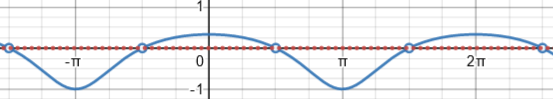
I jumped back in to comment on this asymptote issue:
Hi, Frankie.
I suspect you are confusing the idea of an asymptote (which is a line that the function approaches as you go to infinity) with the related idea of the function being undefined. Many points on a function that are undefined are associated with vertical asymptotes, because the function becomes infinite as it approaches there; but sometimes the graph just has a “hole” because it is undefined at one place, but it remains finite nearby. That is what is happening here. (You have probably seen “holes” in the context of rational functions.)
Here is the original graph in red, including its asymptotes, and the reciprocal graph in blue, showing “holes”.
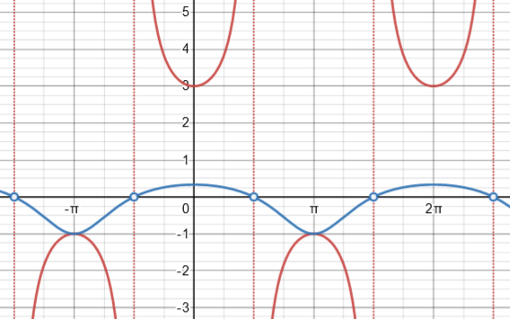
I made a different graph at the time:
The denominator, 1+2 sec(θ), is undefined at these points, so the function 1/(1+2sec(θ)) is likewise not defined there; but the function is approaching 0, not infinity. Here is what the graph really looks like:
(I made this on Desmos, but had to manually add the “holes”, because computers tend not to notice such little details! The open circle represents the fact that one point has been removed from the curve, though points right next to it exist.)
This agrees with your graph. You even included the “holes”, by not letting your graph continue through zero. So you have done well.
I added the explanation of how I made this, as a reminder not to trust a computer too much. It uses a rote method to plot points, without intelligence.
Frankie replied,
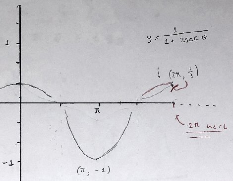
Yes, I was getting confused, I assume then that the reason why there isn’t asymptotes on a finite interval is that they don’t approach infinity. I see now comparing the Desmos graph that it should have a more convex shape as opposed to its concave shape so I have redrawn it in red.
Anyhow thank you both for your help on this question.
Details of the shape, such as convexity, don’t really matter for this problem.
I answered,
Hi, Frankie.
Right. Horizontal asymptotes are relevant only over an unbounded interval. Of course, there could be a vertical asymptote, but there isn’t in this case.
What a horizontal asymptote isn’t
Doctor Rick now added his own comments to both of ours:
Hi, Frankie. If I may join in also, I think there might still be something to clear up about horizontal asymptotes.
Doctor Fenton said,
You cannot have a horizontal asymptote on a finite interval.
You responded with,
If the graph did not have a finite interval would there be an asymptote at y = 0?
Doctor Fenton did not know what you meant by this, but I assume you were asking if there would be a horizontal asymptote of the function y = 1/(1 + 2 sec x) on its full natural domain.
Doctor Peterson talked about confusions regarding asymptotes, which did apply to horizontal asymptotes:
I suspect you are confusing the idea of an asymptote (which is a line that the function approaches as you go to infinity) with the related idea of the function being undefined.
However, he talked mostly about the fact that the function y = 1/(1 + 2 sec x) does not have vertical asymptotes. You then replied:
I assume then that the reason why there isn’t asymptotes on a finite interval is that they don’t approach infinity.
So let me say a bit more about horizontal asymptotes. First, this function is periodic, and a periodic function cannot have a horizontal asymptote. The value of the function does not approach 0, or any other value, as x increases toward infinity; every value in its range continues to appear as its output in each cycle. For instance, y = 1/3 when x = 0, 2pi, 4pi, 6pi, and so on “forever”; but y = -1 when x = pi, 3pi, 5pi, and so on “forever”. It never “settles down”.
Doctor Fenton had mentioned this very briefly.
Second, I wonder if you were thinking that a horizontal asymptote is a horizontal line that never intersects the graph of the function. You might say, Since y never equals zero (though it can get as close to 0 as we want), y = 0 must be a horizontal asymptote. But as Doctor Peterson said, that’s not how to think of an asymptote — it’s all about the graph of the function getting closer and closer to the asymptote as x increases or decreases (for a horizontal asymptote) or as y increases or decreases (for a vertical asymptote).
I may be wrong about what you were thinking, but perhaps this explanation might help you.
The suggestion is that Frankie might be thinking of this as an asymptote, because our function “approaches” it (at certain points) without reaching it:
But a horizontal asymptote involves infinity.
What an asymptote is
Frankie responded:
Yes that does make sense. It seems as though asymptotes are quite closely related to the idea of limits. In that they both arise as the desired input increases/decreases in magnitude. However where an asymptote is essentially “undefined” as the function continues to approach it forever, a limit is “defined” in that it gives us a value the function would, under certain conditions, reach. So they are kind of the converse of each other?
“Converse” is definitely the wrong word! But they can be thought of as the same phenomenon viewed from different directions.
Doctor Fenton finished the discussion with a fuller definition of each kind of asymptote:
Asymptotes aren’t just “related” to limits, they are DEFINED by limits. A vertical asymptote occurs at x=a whenever at least one of the one-sided limits
lim (x→a+) f(x) = ∞ (or -∞) or lim (x→a–) f(x) = ∞ (or -∞) .
That means that the function becomes unbounded in every neighborhood of a. That has nothing to do with whether f(a) is defined or undefined: it is the behavior of f in neighborhoods (a, a+δ) or (a-δ, a) that determines whether a vertical asymptote exists. (In fact, whether f(a) is defined or not has NO effect on whether a limit as x→a exists.) The vertical asymptote is the vertical line x = a. It is not undefined.
In this case, the asymptote is defined by the value of x, which is very much defined!
A horizontal asymptote is defined by a limit at +∞ or at -∞. The horizontal line y = L is a horizontal asymptote of f(x) if either
lim(x→∞) f(x)=L or lim(x→ -∞) = L .
It is also commonly misunderstood that a function graph cannot intersect a horizontal asymptote. That is true for some functions, such as f(x) = 1/x (y = 0 is a horizontal asymptote in both directions) or f(x) = 1/(1+e-x) (y = 1 is a horizontal asymptote as x→∞).
But y = 0 is also a horizontal asymptote for f(x) = e-x sin(x), and f(x) crosses the asymptote infinitely many times.
An ordinary limit tells you about the behavior of a function as x gets nearer and nearer to a point, but it tells you NOTHING about f(a) itself. f(a) may exist or not; it does not affect whether f has a limit at a.
A horizontal asymptote tells you about the behavior of a function for ever increasing values of x.