Last week’s discussion about zeros of a polynomial, and other conversations, have reminded me of a past discussion of the shape of the graph of a polynomial near its zeros. Let’s take a look, starting with some other questions that nicely lead up to it.
High multiplicity: Flatness
We’ll start with this question from 1997:
Root Multiplicity and Polynomial Functions

What effect does multiplicity have on a polynomial function?

Here's an example of what I mean by multiplicity: (x+1)(x-2)^2 where -1 has a multiplicity of 1 and 2 of 2.

I can't figure out what effects multiplicities have, although odd multiplicities appear to make the function parallel to the x axis for a while, like x(x-2)^9. But 3 is not parallel to the x axis, nor is 1. The higher the multiplicity, the farther the function appears to travel along the x axis, but only up to a point.

Can someone please help?
The multiplicity of a zero of a polynomial is the degree of the corresponding factor; if there is a factor \((x-a)^m\), then we say that a is a zero of multiplicity m. When the multiplicity is 1, the graph crosses straight through the x-axis, but for higher multiplicities, it briefly flattens out, as Alex has observed.
Here are the graphs of Alex’s two functions:
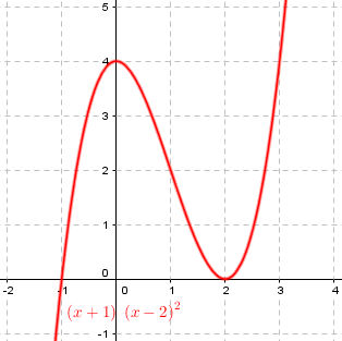
There, the zero of multiplicity 2, at \(x=2\), is momentarily horizontal, touching the x-axis (and then turning back, as we’ll see, because 2 is even).
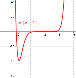
With multiplicity 9, again at \(x=2\),, it appears to be (nearly) horizontal for some distance (most of the way from \(x=1\) to \(x=3\), as he pointed out); it is actually horizontal only momentarily, but is very close to horizontal for much farther. (Then it crosses over, because 9 is odd.)
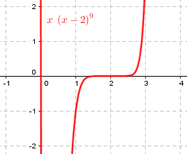
It still looks pretty horizontal (though not quite as far) if we don’t stretch the scale vertically:
Doctor Jerry answered:
Hi Alex,

You have done well in thinking about the effect on the graph of multiple roots.

If y = q(x)*(x-a)^k, where q(x) is the rest of the polynomial we are considering, if k is large, then the factor (x-a)^k will be very small within 1 of a. This means that the graph will be quite flat in the interval (a-1,a+1). Of course, if k is only 1 or 2, the flatness is limited to a short interval about a.
The idea is that when \(|x-a|\) is less than 1, raising it to a power will make it smaller. Closer to a, this factor will be very small; for instance, for \(|x-a|<0.5\), \(|x-a|^9<0.002\). So it is, indeed, very flat. Lower powers are less effective; for \(|x-a|<0.5\), \(|x-a|^2<0.25\), but it is still flat when you get closer: for \(|x-a|<0.05\), \(|x-a|^2<0.0025\). This matches what we see on the graphs.
Note that when \(k=1\), there is really no flattening at all; that was an accidental misstatement.
When k is even, the factor (x-a)^k doesn't change sign as x moves from the left of a to the right of a (assuming that q(x) doesn't have roots very close to a). So, the graph will be tangent to the x-axis. For odd k, the graph crosses the x-axis, even though it may be quite flat.
For even multiplicity, books often say the graph “touches and turns“, being either positive on both sides, or negative on both sides. For odd multiplicity, it “crosses“; I describe it as “pausing before continuing in the same direction”.
Odd and even multiplicity: Touching vs crossing
Here is a related question from 2004:
Graphing Polynomial Functions in Factored Form

Why does even multiplicity cause a graph to touch an intercept and odd multiplicity cause a graph to cross it?
We saw this in the first graph above, where the zero at \(x=-1\) had odd multiplicity (1) and crossed the x-axis from above to below, while the zero at \(x=2\) had even multiplicity (2) and touched from above without crossing. But we only “touched” on this fact there.
Doctor Vogler answered:
Hi Shannon,

Thanks for writing to Dr Math.  Suppose we have a polynomial

  f(x) = (x - r)^m * (other terms)

with a root r of multiplicity m.  So the other terms are not near zero when x is near r.  That is, if you look close enough to r, the other terms will be close to some nonzero number, either positive or negative.  Or, said differently, the limit as x approaches r of those other terms is some nonzero real number.  If it was zero, then we could factor out another x - r from those other terms, and the root r would have multiplicity m + 1.
He is using the word “term” where I would say “factor”; the main point is that the multiplicity must be the highest degree you can put on that factor, so the “other terms” (Doctor Jerry’s \(q(x)\)) will not be zero at r, and will be close to some non-zero number anywhere near r.
For example, if our function is $$f(x)=x(x+1)^2(x-2)^3$$ and we are focusing on the zero at \(x=-1\), with multiplicity 2, we are looking at it as $$f(x)=\left[x(x-2)^3\right](x+1)^2$$ so that the “other terms” are \(x(x-2)^3\), which is near \((-1)((-1)-2)^3=27\) when x is near \(-1\). Here is the graph, which crosses the axis at \(x=0\) and at \(x=2\), but only touches at \(x=-1\):
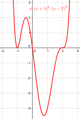
So then when x = r, f(x) = f(r) = 0.  That causes the graph to touch the x-axis at (r,0).  Now when x is just larger than r (that is, just to the right of r), then x-r will be positive, and (x-r)^m will also be positive.  So f(x) will have the same sign as the product of those other terms.

But when x is just smaller than r, then x-r will be negative, and (x-r)^m might be negative and might be positive.  In fact, (x-r)^m will be negative if m is odd, and (x-r)^m will be positive if m is even.  So if m is even, then f(x) will have the same sign as those other terms, which means it approaches the 0 at f(r) but has the same sign on both sides of r, so it touches and does not cross.  But if m is odd, then f(x) will have the opposite sign as those other terms, which means it has a different sign on each side of r, so it crosses the axis.
He hasn’t explicitly talked here about the flattening aspect (for multiplicities greater than 1), just the sign aspect. We’ll put everything together next.
But just what shape does it have?
Here is the question I find most interesting, from 2014:
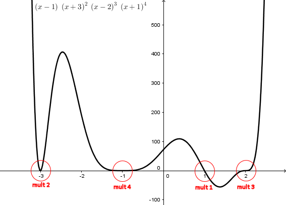
Curvy ... and Topsy-Turvy?

When sketching curves of higher degree polynomials, we can use factorisation to look at the parts of the equation that make up the whole polynomial. Therefore, we can look at the curve in terms of smaller curves, especially on the x-axis (the roots).

For example, consider the function

   y = (x - 1) * (x + 3)^2 * (x - 2)^3 * (x + 1)^4

Its curve will cross the x-axis like a linear function at 1, like a parabola at -3, like a cubic at 2, and like a quartic at -1. When we do this, we get the shape of the curve. It begins in the first quadrant and ends in the second because it is positive.

But when we look at the roots of the equation, the linear function formed at (1, 0) looks like the equation y = -x - 1 (negative) rather than y = x - 1 (as in the original term).

Why is this?

Even though the original term was (x - 1), the graph of the entire function looks negative near x = 1. Similarly, in other regions, the signs of the roots seem opposite to the roots of the individual terms.

What part of the equation determines this?
Here is the graph of his function, with the zeros marked:
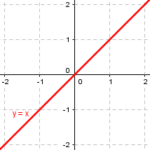
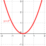
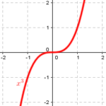
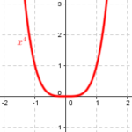
What Sam has been taught, evidently, is that near an x-intercept (zero, or root), a polynomial behaves in some sense like a polynomial whose degree matches the multiplicity of the zero (the exponent on the corresponding factor). Here are graphs of polynomials of first, second, third, and fourth degree, for comparison:
But what does “like” mean?
Doctor Greenie answered, taking “like” to mean “exactly like”, according to Sam’s evident expectation:
Hi, Sam --

What you are saying is not true at all.

The factorization of the polynomial tells us where the roots are, and the powers of the factors tell us the general behavior of the function at the zeros.

But it appears that you are saying that the function in your example, because of the factor (x - 1), should look like the linear function y = x - 1 at x = 1.

That is not at all true. If it were, then the slope of the function at every zero would be positive, because the factors are all of the form (x - a), not (-x - a), and that would not be possible.
As Sam had observed, the function does not look like the corresponding power function in this sense.
Digging deeper
I, writing at the same time, saw “like” more broadly:
Hi, Sam.

An excellent question!

Let's look at the factor (x - 1) in its context:

   y = (x - 1) * (x + 3)^2 * (x - 2)^3 * (x + 1)^4
        =====

Since we're looking at the curve NEAR x = 1, all the other factors will be near the value they take at x = 1. (A small change in x will produce a large relative change in (x - 1), since it is near zero, but only a small relative change in the other factors.) If we replace x with 1 in those other factors, we have

   y ≈ (x - 1) * (1 + 3)^2 * (1 - 2)^3 * (1 + 1)^4
     = (x - 1)(16)(-1)(16)
     = -256(x - 1)

That factor of -256 answers your question. The specific linear function that approximates the curve near x = 1 is y = -256(x - 1), with a negative slope.
I’m not sure I had ever taken the idea quite this far before. But it was implied in the other two answers above, if I had thought about it.
Here is what this linear function looks like, in comparison to the polynomial:
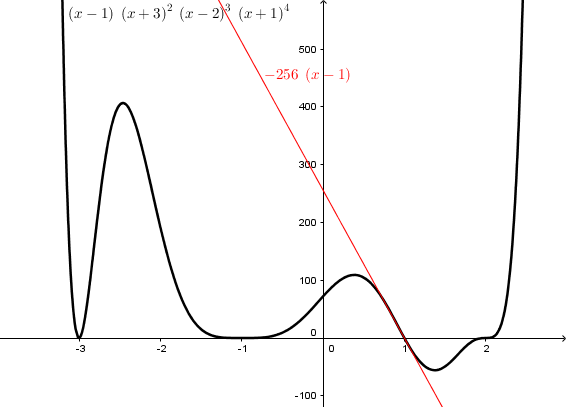
This line is tangent to the curve; if you zoomed into the graph, it would look almost identical.
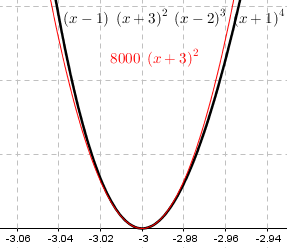
Similarly, if we replace x in all factors except \((x+3)^2\) with \(-3\), we get \(y=8000(x+3)^2\), which looks like this:
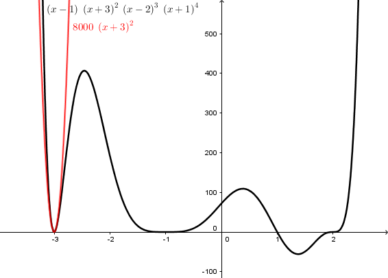
This is not only tangent to the curve (that is, horizontal) at the given point, but remains close for points nearby; here is what it looks like if we zoom in:
Here are the results if we do the same with the other two zeros:
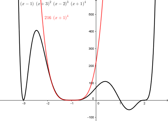
You can see that the flatness at \(-1\) is because \(y=(x+1)^4\) is flattened. Multiplying by 216 doesn’t change that much.
I wanted to let him do this for himself … but then I couldn’t resist showing my results in case he didn’t:
Try doing the same with the other x-intercepts, and graph these approximations on the same axes as the curve. I think you'll like what you see!

Here is my graph:
After seeing Doctor Greenie’s answer, I added more:
Hi, Sam.

I have a clarification to make.

I tell my students that a polynomial near any zero h "looks like" the corresponding factor (x - h)^n, in the broad sense that if the factor is cubed, it looks like a cubic, and so on. This is what you said initially ("like a cubic"). A cubic, of course, can look either like x^3 or like -x^3, which is where your question arose.
So the issue is what we mean by “a” cubic, more than on the meaning of “looks like”.
In a more exact sense, it looks like a(x - h)^n, where the coefficient "a" has to be determined as I showed you, by putting x = h into the other factors. If you want to get the direction right, as well as the overall shape, you have to at least determine the sign of this coefficient.
This amounts to finding the sign of the entire polynomial for x slightly greater than the zero, which determines the effective “leading coefficient”.
So the answer to your specific question -- about what part of the expression determines the direction -- is: "all the rest."
So we are back to the “other terms” we’ve been seeing all along.
Osculating curves: defining “close” by calculus
The factor of interest determines the degree of the shape we are looking for, and the sign of all the other factors determines the direction of the shape. This is the same as the “other terms” or “q(x)” mentioned in the first two answers. I continued:
The graph I shared yesterday showed this for all four zeros, carrying out the plan I suggested. Note how, with the coefficients calculated correctly, the graph looked very much like the corresponding functions; in fact, no polynomial could more closely "snuggle up to" the curve at those points than these. They are called "osculating curves" (from the Latin for "kiss"):

    http://mathworld.wolfram.com/OsculatingCurves.html
That page says osculating curves have the same value, first derivative, and second derivative at the given point, so that they have the same location, slope, and curvature. Let’s check that out for our example at \(x=2\); this will require a little calculus:
$$f(x)=(x-1)(x+3)^2(x-2)^3(x+1)^4\\=x^{10}+3x^9-13x^8-37x^7+57x^6+157x^5-71x^4-279x^3-46x^2+156x+72$$
$$f'(x)=10x^9+27x^8-104x^7-259x^6+342x^5+785x^4-284x^3-837x^2-92x+156$$
$$f^{\prime\prime}(x)=90x^8+216x^7-728x^6-1554x^5+1710x^4+3140x^3-852x^2-1674x-92$$
$$f^{\prime\prime\prime}(x)=720x^7+1512x^6-4368x^5-7770x^4+6840x^3+9420x^2-1704x-1674$$
At \(x=2\),
$$f(2)=(2)^{10}+3(2)^9-13(2)^8-37(2)^7+57(2)^6+157(2)^5-71(2)^4-279(2)^3-46(2)^2+156(2)+72=0$$
$$f'(2)=10(2)^9+27(2)^8-104(2)^7-259(2)^6+342(2)^5+785(2)^4-284(2)^3-837(2)^2-92(2)+156=0$$
$$f^{\prime\prime}(2)=90(2)^8+216(2)^7-728(2)^6-1554(2)^5+1710(2)^4+3140(2)^3-852(2)^2-1674(2)-92=0$$
$$f^{\prime\prime\prime}(2)=720(2)^7+1512(2)^6-4368(2)^5-7770(2)^4+6840(2)^3+9420(2)^2-1704(2)-1674=12,150$$
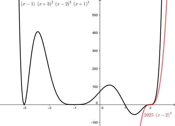
Those all agree with the derivatives of \(g(x)=2025(x-2)^3\), whose first three derivatives are
$$g'(x)=6075(x-2)^2\;\;\;g'(2)=0$$
$$g^{\prime\prime}(x)=12,150(x-2)\;\;\;g^{\prime\prime}(2)=0$$
$$g^{\prime\prime\prime}(x)=12,150\;\;\;g^{\prime\prime\prime}(x)=12,150$$
So our cubic “hugs” as tightly as a polynomial possibly can: All its derivatives match at that point. We might call it a “hyper-osculating” curve.
And we can easily see why, if we use the product rule to find the derivatives:
$$f(x)=\left[(x-1)(x+3)^2(x+1)^4\right]\cdot(x-2)^3$$
$$f'(x)=\left[\text{6th degree polynomial}]\right]\cdot(x-2)^3+\left[\text{7th degree polynomial}\right]\cdot3(x-2)^2$$
which is zero at \(x=2\);
$$f^{\prime\prime}(x)=\left[\text{5th degree polynomial}]\right]\cdot(x-2)^3+\left[\text{6th degree polynomial}]\right]\cdot3(x-2)^2\\+\left[\text{6th degree polynomial}\right]\cdot3(x-2)^2+\left[\text{7th degree polynomial}]\right]\cdot6(x-2)$$
which is zero at \(x=2\), because every term has \(x-2\) as a factor.
Then the next derivative will have one term that does not have that factor; since that “7th degree polynomial” is just the “other terms” \((x-1)(x+3)^2(x+1)^4\), it will be $$f^{\prime\prime\prime}(x)=\left[\text{stuff with }(x-2)\right]+\left[(x-1)(x+3)^2(x+1)^4\right]\cdot6$$ and $$f^{\prime\prime\prime}(2)=\left[(2-1)(2+3)^2(2+1)^4\right]\cdot6=2025\cdot6=12,150$$ just as before.