
Last time, we saw a summary of the difference between population and sample standard deviation, along with other differences in formulas. Here we’ll look at two short answers about the reason for that difference, and then an extensive look at why it’s true. (I’ve taken extra time and space to work through details in order to convince myself, and hopefully save you that time!)
Why use n – 1 for a sample?
Here is the second part of a 1995 question, the first part of which we answered two posts ago:
Questions About Standard Deviation

2.  What is the reasoning behind dividing by n vs. n-1 in the population versus sample standard deviations?
Let’s see Doctor Steve’s answer:
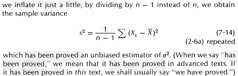
2. The reason that n-1 is used instead of n in the formula for the sample variance is as follows: The sample variance can be thought of as a random variable, i.e. a function which takes on different values for different samples of the same distribution. Its use is as an estimate for the true variance of the distribution. In statistics, one typically does not know the true variance; one uses the sample variance to ESTIMATE the true variance. Since the sample variance is a random variable, it usually has a mean, or average value. One would hope that this average value is close to the actual value that the sample variance is estimating, i.e. close to the true variance. In fact, if the n-1 is used in the defining formula for the sample variance, then it is possible to prove that the average value of the sample variance EQUALS the true variance. If we replace the n-1 by an n, then the average value of the sample variance is ((n-1)/n) times as large as the true variance.
Another way to say this, in line with some of our previous answers, is that in order to use the variance of a sample as an estimate for the population, the variance of the sample, initially defined using the n, has to be corrected by multiplying it by \(\frac{n}{n-1}\). This is called Bessel’s correction.
A random variable X which is used to estimate a parameter p of a distribution is called an unbiased estimator if the expected value of X equals p. Thus, using the n-1 gives an unbiased estimator of the variance of a distribution.
And using n (to find the standard deviation of the sample in itself) gives a biased estimator.
More on unbiased estimators
A 2006 question asked the same question and got a deeper answer:
Difference in Standard Deviation Formulas

In regards to sample vs. population standard deviation, why is (n-1) used in the denominator rather than n?
Doctor Wilko answered:
Hi Stefan,

Thanks for writing to Dr. Math!

The answer would be found in any graduate-level book on probability. You would have to look up topics on biased/unbiased estimators.

The first question for us to answer is "What's an estimator?".

Definition:  An estimator is a rule/formula that tells us how to calculate the value of an estimate based on the measurements contained in the sample.
As in the previous answer, at an introductory level we can really only say “it can be proved …” (in more advanced books). We have no idea what Stefan has learned. But he’ll try explaining the concept.
Let's think about this using means (averages).

For example, if we take a random sample of 20 test scores from a class of 35 students, we can try to estimate the entire class average (population mean) by calculating the sample mean from these 20 scores.  This sample mean is an estimator of the true population mean.  The rule/formula in this example is to take the 20 scores, add them up, and divide by 20.  The answer we get, the sample mean, is an estimator--our best inference about the true population mean (which we don't know, that's why we're trying to estimate it).

Now that we know what an estimator is, the short answer to your question is that sample variance (an estimator) COULD'VE been defined as "the sum of the squares of each value minus the sample mean divided by n", but it turns out that this is a BIASED estimator.
It can be shown (as we’ll see later) that the sample mean is an unbiased estimator of the population mean, meaning that the average of all possible sample means matches the mean of the population, so that if the sample is representative of the population, it will probably be close, even though it will never be exact. That isn’t true of the naive sample standard deviation:
So, what's a biased estimator?

A biased estimator in this case means that the sample variance calculated this way (divided by n) underestimates the true population variance.  If we are trying to make an inference about the true population variance, we don't want to underestimate, we want to be as accurate as we can!

So, using some theory from probability, it can be shown that this biased sample variance (as defined by dividing by n) can be made UNBIASED by dividing by (n-1) instead.

So, that's the reason we divide by (n-1)--to get an unbiased estimator.  Now we have a good estimator that we can use when making inferences about a population!
By the way, it turns out that the sample standard deviation, even with its correction, is technically not an unbiased estimator of the population standard deviation; but the sample variance is an unbiased estimator of the population variance! That’s because of how square roots work. So we just do the best we can using the variance.
Can we prove it simply?
Back in 1999, a question from Italy led to a very long discussion that will take up the rest of our space:
Estimators of Statistics Variables

I'm interested in the properties of the estimators for the most common values in statistics and I have some questions:

Let s^2 = sum((Xi-M)^2)/n and sigma^2 = sum((Xi-M)^2)/(n-1). Is there an elementary proof that s^2 of a sample in not an unbiased estimator for s^2 of the population while sigma^2 of a sample is an unbiased estimator for sigma^2 of the population?
(I’m omitting another question, about the median as an estimator for the mean, for the sake of space.)
The question is slightly misleading: He seems to have swapped the two formulas; and also, in my experience at least, the symbol \(s^2\) is used only of a sample and \(\sigma^2\) of the population. It is \(s^2\) (the adjusted form with \(n-1\)) that is an unbiased estimator of \(\sigma^2\). Perhaps some of this is different in Italy, or in his textbook.
After Doctor Mitteldorf tried to answer in a way that turned out not to be helpful, which I will also omit, In response, Eugenio presented his own ideas, which I’ll present as an answer rather than a question:
Dear colleague,

I thank you very much for your kind reply to my request; what you suggest is really interesting, but I'm trying something different. I've only basic knowledge in statistics, I teach math in an Italian high school (to 18-year-old students) and I just wanted to show them why in scientific calculators there are two different keys for the standard deviation: "sx" and "sigmax."
So a common calculator has buttons labeled \(sx\) for the adjusted form (sample), and \(\sigma x\) for the n form (population), and he wants, if not a full proof, at least a high-school level justification for the difference.
Now he presents his own attempt, which doesn’t work.
Here is what I have in mind:

Suppose we have a population of n people and each person is associated with a particular value Xi where i = 1, 2, ..., n (e.g. his weight).

Let
   MP = sum(Xi)/n be the arithmetic mean of the population,
and
   SIGMA^2P = sum((Xi-M)^2)/n and
   S^2P = sum((Xi-M)^2)/(n-1)
be two possible definitions for the population variance.

Let's take k elements (k < n) to form a sample and let's define MS, SIGMA^2S, and S^2S to be the analogue values calculated on the chosen sample.

If we imagine calculating these values for all the possible C(n,k) (combinations of n objects taken k at a time) samples, these values become random variables each one with its particular mean value; if X is a random variable, let's call E(X) (E = Expectation) its mean value.
This is a good beginning. His \(S^2_P\), using \(n-1\) for the population, is never actually used; his \(\sigma^2_S\) is the mean square deviation (uncorrected variance) for a sample, and \(S^2_S\) is the (corrected) variance for the sample, commonly called the “sample variance”. And he’s exactly right in treating the variance of a sample as a random variable in its own right. We want its mean (expectation) to be \(\sigma^2_P\), and that will be the average over all the possible samples.
We say that MS is an "unbiased" estimator of MP because E(MS) = MP (and this is easy to prove).

One could expect SIGMA^2S to be an unbiased estimator for SIGMA^2P, but this is not true: in order to have unbiased estimators you have to substitute SIGMA^2P with S^2P and SIGMA^2S with S^2S.
Yes, the expected value of the sample means is the population mean. Let’s prove it:
In averaging all \(C(n,k)\) sample means, you are adding the sums of that many sets of k numbers, adding \(kC(n,k)\) numbers, and therefore including each of the n elements of the population \(\frac{k}{n}C(n,k)\) times, giving a sum of \(\frac{kC(n,k)\sum x}{n}\).
So the sum of the sample means (dividing by k) is \(\frac{C(n,k)\sum x}{n}\).
On dividing by \(C(n,k)\) to get the average of those means, you would obtain \(\frac{\sum x}{n}\), which is the mean of the population.
What he says about the variance is a little off; we will find that \(E\left(S^2_S\right)=\sigma^2_P\), so it is only for the sample that we use \(S\) instead of \(\sigma\).
Here is a numeric example: let's take a population of n = 4 elements and the values 1, 2, 4, 13. We have MP = 5, SIGMA^2P = 90/4 = 45/2, S^2P = 90/3 = 30 related to the whole population.

Suppose we take samples of k = 3 elements. If we sample without replacement, we have C(4,3) = 4 possible samples; for each sample let's calculate MS, SIGMA^2S and S^2S:

     SAMPLE      MS    SIGMA^2S    S^2S
     ------      --    --------    ----
     1, 2, 4     7/3      14/9      7/3
     1, 2, 13   16/3     266/9    133/3
     1, 4, 13    6        26       39
     2, 4, 13   19/3     206/9    103/3

Each sample has the same probability 1/4, calculating the mean value of the three random variables we have: E(MS) = 5, E(SIGMA^2S) = 20, and E(S^2S) = 30.
An example like this is excellent for understanding without a formal proof; and what he’s done here is correct as far as he goes. (I’ll be doing the same below with a more interesting little population.)
Observe that the average of the sample means is $$\frac{1}{4}\left[\frac{7}{3}+\frac{16}{3}+\frac{18}{3}+\frac{19}{3}\right]=\frac{7+16+18+19}{12}=5,$$ and this not only is the population mean, but must be so, because the numerator, \(7+16+18+19\), is $$(1+2+4)+(1+2+13)+(1+4+13)+(2+4+13)\\=1+1+1+2+2+2+4+4+4+13+13+13,$$ which is 3 times the sum of the population. This illustrates our little proof.
But he’s found the expected values of the unadjusted and adjusted variances of the sample, and found that they are 20 and 30, respectively, and not 22.5 as we wanted. So it didn’t work. (He did find that his \(E(S^2_S)=S^2_P=30\); I’m not sure if that is generally true, and since it is not a true variance, it is not helpful.)
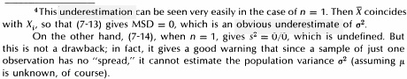
While E(MS) = MP and E(S^2S) = S^2P, E(SIGMA^2S) <> SIGMA^2P and the variance SIGMA^2S is not an unbiased estimator for SIGMA^2P. Note that, for any population and for any "n", if we take k = 1, SIGMA^2S of any sample is 0 (while S^2S is not defined: 0/0) so,

     E(SIGMA^2S) = 0 <> SIGMA^2P

and that is enough to prove that SIGMA^2S cannot be an unbiased estimator for the variance of the entire population. As you see, these statements are very general and not connected to the population distribution (they're always true).
Since the claim can’t be true for a sample of 1, how can it be called true in general? As we’ll see, he’s missed only one detail: For the proof, we’ll need to sample with replacement. The reality is that samples without replacement can only approximate the population variance for very large populations, for which replacement makes negligible difference.
In the Italian translation of "Introductory Statistics" by T. H. Wonnacott and R. J. Wonnacott, I read "it is possible to demonstrate that S^2S is an unbiased estimator for S^2P, the demonstration can be found in more complete books." I just wonder how difficult this demonstration could be. (Can you tell me something about it?)
Although I don’t have access to this book, I was able to find a snippet that says, “But if …
I also found a footnote that mentions the \(k=1\) case:
Trying for an understandable proof
Now Doctor Mitteldorf got some help:
Dear Eugenio,

I consulted with a colleague here at the Math Forum, Doctor Anthony, who has helped me see the proof of your statement that the variance of the sample multiplied by (n/n-1) is an unbiased estimator for the variance of the set from which the sample is drawn. Here's the proof, based on his explanation to me.
Note that, as we’ve seen before, they are defining variance itself using the division by n, and thinking of what is often described as sample variance as an adjustment to that, for the purpose of estimating (Bessel’s correction).
Note also that none of us can answer every question; one of the benefits of Ask Dr. Math was having a variety of colleagues with different strengths! (There are fewer now.) It’s also worth noting that we will not be making a mathematically complete proof; Doctor Anthony emphasized intuitive thinking rather than formal perfection. That’s just what we were hoping for. But it will still require some careful thought.
First, some notation:

"Global average" means average over the entire, large set from which the samples are drawn. I'll write global averages as {F}.

"Sample average" is the average of one sample of n drawn from the large set with replacement. I'll write sample average as <F>.

"Ensemble average" is the average over a large number of samples of size n, and I'll write the ensemble average as [F]. The ensemble is assumed to be large enough that [<x>] = {x}, i.e. the mean of a large number of sample means is the same as the global mean.
The global average, “\(\{\dots\}\)”, is the average of the population.
The sample average, “\(\left<\dots\right>\)”, is the average of a single sample.
The ensemble average, “\([\dots]\)”, we can think of as the mean taken over every possible sample! At least, that’s what we’re approaching as we take more and more samples.
To take a very small example, suppose the population consisted of \(P=\{1,2,2,5\}\). Then the global mean would be $$\{P\}=\frac{1+2+2+5}{4}=2.5.$$ (I’ve intentionally included the value 2 twice in the population, to be sure we take that possibility into account; Eugenio’s example avoided this, so it’s helpful to do both.)
For one sample of 2, \(S=\{1,2\}\), the sample mean would be $$\left<S\right>=\frac{1+2}{2}=1.5.$$
There are 16 equally likely possible samples of 2 with replacement (thought of here as ordered pairs), namely $$E=\{(1,1),(1,2),(1,2),(1,5),\\(2,1),(2,2),(2,2),(2,5),\\(2,1),(2,2),(2,2),(2,5),\\(5,1),(5,2),(5,2),(5,5)\},$$ with respective sample means $$1,1.5,1.5,3,\\1.5,2,2,3.5,\\1.5,2,2,3.5,\\3,3.5,3.5,5,$$ so the ensemble mean of all these samples is $$[E]=\frac{1+1.5+1.5+3+1.5+2+2+3.5+1.5+2+2+3.5+3+3.5+3.5+5}{16}=\frac{40}{16}=2.5$$ This is equal to the population mean, illustrating that general fact. More generally, a sufficiently large set of random samples, with replacement, should be close to this.
Moreover, if the population itself is large, replacement shouldn’t make much difference. (Real samples are made without replacement, but it is easier to calculate with replacement.) This will be the key to the success of this proof, in contrast to Eugenio’s.
But what we want to explore is the variance, which applies these ideas to squares; specifically, in these terms, the variance of a population is \(\{x^2\}-\{x\}^2\), the (global) average of all squares minus the square of the average. We want to show that we can estimate this using the variance of a sample, because the (ensemble) average of all such sample variances, after an adjustment will be the variance of the population. The average of sample variances (without the correction) is $$\left[\left<x^2\right>-\left<x\right>^2\right].$$ So what we want to show is that $$\left[\left<x^2\right>-\left<x\right>^2\right]\cdot\frac{n}{n-1}=\left\{x^2\right\}-\left\{x\right\}^2,$$ or equivalently $$\left[\left<x^2\right>-\left<x\right>^2\right]=\frac{n-1}{n}\left(\left\{x^2\right\}-\left\{x\right\}^2\right).$$ This last line is the theorem we’ll be proving.
Proving a lemma
Next, a lemma: It's a familiar result that the means of samples of size n have a variance (1/n) times the global variance. In my notation:

     [<x>^2] - [<x>]^2 = (1/n)({x^2} - {x}^2)

The meaning is: take a random sample of size n (with replacement). Calculate the sample mean. Repeat this again and again, until you have a large number of such mean values. The variance of this ensemble is (1/n) times the variance of the global set from which the samples are drawn.
Recall the last formula we worked out last time: $$\sigma^2=\mathrm{E}\left(x^2\right)-\left(\mathrm{E}\left(x\right)\right)^2=\left\{x^2\right\}-\left\{x\right\}^2.$$ That’s the global variance; and the variance of sample means is found by replacing x with \(\left<x\right>\), and global means with ensemble means.
So the lemma says that $$\left[\left<x\right>^2\right]-\left[\left<x\right>\right]^2=\frac{1}{n}\left(\left\{x^2\right\}-\left\{x\right\}^2\right).$$
This looks a lot like what we want to prove; look carefully to see the differences! The LHS is the (ensemble) variance of the sample means; the RHS is the (global) variance of the population, divided by the sample size.
You may have used the fact that the variance of sample means is \(\frac{\sigma^2}{n}\). or, equivalently, that the standard deviation of sample means is \(\frac{\sigma}{\sqrt{n}}\); that’s what this says. One implication is that the larger the sample, the closer you can expect its mean to be to the population mean.
But this needs to be proved:
Proof of the lemma: We may assume without loss of generality that the distribution is centered about zero, i.e. {x} = 0. Then it will also be true that [<x>] = 0, as we noted above. So we are left with

     [<x>^2] = (1/n){x^2}
We’re proving the lemma only for the case where the mean of the population is 0; you can check for yourself that if we add some number to all the x‘s to change the mean, the lemma will still be true. (Variance is not affected by a shift of all the data.) That’s what “without loss of generality” means.
So the lemma in this case reduces to $$\left[\left<x\right>^2\right]=\frac{1}{n}\left\{x^2\right\},$$ and that’s what we want to prove.
On the left, we have the average of a large number of terms, each of which is

     ((1/n)*SUM(xi))^2

This can be written as

     (1/n^2)*(SUM(xi^2)+SUM(2xi*xj))
So the mean of the squared means of the samples (the LHS) is the mean of terms $$\left<x\right>^2=\left(\frac{1}{n}\sum_{i=1}^n x_i\right)^2$$ and much as we did last time in proving the equivalence of the shortcut formula, we can expand this: $$\left(\frac{1}{n}\sum_{i=1}^n x_i\right)^2=\left(\frac{1}{n}\right)^2\left(\sum_{i=1}^n x_i\right)\left(\sum_{j=1}^n x_j\right)\\=\frac{1}{n^2}\left(\sum_{i=1,j=1}^n x_ix_j\right)=\frac{1}{n^2}\left(\sum_{i=1}^n x_i^2+2\sum_{i<j} x_ix_j\right),$$ where the last step separates pairs i, j into cases with the same index, and cases with unequal indices. Each pair of distinct indices appears twice in the sum, once with \(x_i\) smaller, and once with \(x_i\) larger.
For example, if \(n=3\), then what we have for any given sample is $$\left<x\right>^2=\left(\frac{1}{3}\left(x_1+x_2+x_3\right)\right)^2=\frac{1}{9}\left(x_1+x_2+x_3\right)\left(x_1+x_2+x_3\right)\\=\frac{1}{9}\left(x_1x_1+x_1x_2+x_1x_3+x_2x_1+x_2x_2+x_2x_3+x_3x_1+x_3x_2+x_3x_3\right)\\=\frac{1}{9}\left(x_1^2+x_2^2+x_3^2+2x_1x_2+2x_1x_3+2x_2x_3\right)\\=\frac{1}{9}\left(\left(x_1^2+x_2^2+x_3^2\right)+2\left(x_1x_2+x_1x_3+x_2x_3\right)\right)$$
Now we’re averaging these expressions over many (or ultimately, all possible) samples. This will amount to summing all products of pairs of data values in the population:
The second sum is over cross-terms of the form xi*xj, with i ≠ j. When we take the ensemble average of these terms, they go to zero because

     SUM(xi) = 0

(Note that the sample is with replacement, so it is not necessarily true that xi ≠ xj. The sum over a large number of pairs xi*xj will be zero because it is a multiple of SUM(xi), which by assumption is zero.)
That is, when we add up all these sums of products of distinct values from samples, each x is multiplied by every other x, and since we assume their mean is 0, so is their sum. I found this difficult to convince myself of (in part because a typo in this paragraph made me unsure whether I was reading it correctly!), so I’ll dig into this.
Back to an example
To see better what is happening here, consider my example population from above. To be able to apply the reasoning here, we need to make the mean zero, which we can do by subtracting the mean, so our new population is \(\{-1.5,-0.5,-0.5,2.5\}\). Again we have 16 possible samples of two; so the LHS of the lemma (ensemble mean of squared sample means) is
$$\left[\left<x\right>^2\right]=\frac{1}{16}\left[\left(\frac{-1.5-1.5}{2}\right)^2+\left(\frac{-1.5-0.5}{2}\right)^2+\left(\frac{-1.5-0.5}{2}\right)^2+\left(\frac{-1.5+2.5}{2}\right)^2\\+\left(\frac{-0.5+-1.5}{2}\right)^2+\left(\frac{-0.5+-0.5}{2}\right)^2+\left(\frac{-0.5-0.5}{2}\right)^2+\left(\frac{-0.5+2.5}{2}\right)^2\\+\left(\frac{-0.5-1.5}{2}\right)^2+\left(\frac{-0.5-0.5}{2}\right)^2+\left(\frac{-0.5-0.5}{2}\right)^2+\left(\frac{-0.5+2.5}{2}\right)^2\\+\left(\frac{2.5-1.5}{2}\right)^2+\left(\frac{2.5-0.5}{2}\right)^2+\left(\frac{2.5-0.5}{2}\right)^2+\left(\frac{2.5+2.5}{2}\right)^2\right]=\\\frac{1}{64}\left[\left(-3\right)^2+\left(-2\right)^2+\left(-2\right)^2+\left(1\right)^2+\left(-2\right)^2+\left(-1\right)^2+\left(-1\right)^2+\left(2\right)^2\\+\left(-2\right)^2+\left(-1\right)^2+\left(-1\right)^2+\left(2\right)^2+\left(1\right)^2+\left(2\right)^2+\left(2\right)^2+\left(5\right)^2\right]\\=\frac{1}{64}\left[9+4+4+1+4+1+1+4+4+1+1+4+1+4+4+25\right]=\frac{72}{64}=\frac{9}{8}$$
The RHS of the lemma is $$\frac{1}{n}\left\{x^2\right\}=\frac{1}{2}\cdot\frac{1}{4}\left[\left(-1.5\right)^2+\left(-0.5\right)^2+\left(-0.5\right)^2+\left(2.5\right)^2\right]=\frac{1}{8}\left[2.25+0.25+0.25+6.25\right]=\frac{9}{8}$$
So the lemma is true.
How does this relate to the proof?
For one sample, say \((-1.5,-0.5)\), we have $$\left<x\right>^2=\left(\frac{-1.5-0.5}{2}\right)^2=\frac{1}{4}\left(-1.5-0.5\right)^2=\frac{1}{4}\left(\left(-1.5\right)^2+2\left(-1.5\right)\left(0.5\right)+\left(0.5\right)^2\right)$$
When we average a large number of such samples, we will be adding many squares (the first and last terms) and also many products of distinct data values. For my example, when we average all squared sample means, the sum of all products is $$(-1.5)(-1.5)+(-1.5)(-0.5)+(-1.5)(-0.5)+(-1.5)(2.5)\\+(-0.5)(-1.5)+(-0.5)(-0.5)+(-0.5)(-0.5)+(-0.5)(2.5)\\+(-0.5)(-1.5)+(-0.5)(-0.5)+(-0.5)(-0.5)+(-0.5)(2.5)\\+(2.5)(-1.5)+(2.5)(-0.5)+(2.5)(-0.5)+(2.5)(2.5)\\=2.25+0.75+0.75-3.75+0.75+0.25+0.25-1.25\\+0.75+0.25+0.25-1.25-3.75-1.25-1.25+6.25=0$$
Note that these are products of distinct data values from samples, not necessarily different data values; this is the point of his comment that \(i\ne j\) does not imply that \(x_i\ne x_j\), because the sampling is with replacement, but also because, as I intentionally did in my example population, a population can contain repeat values.
That means that the cross terms are products of two distinct values in any given sample, which includes samples in which the same value was taken twice (because of sampling with replacement). The numbers in each product have distinct indices in a sample, not necessarily in the population from which it is taken. So the ensemble sum includes each number multiplied by every number, including itself, and since the sum of all the numbers is zero, so is this sum of products, just as we see in the example. You can see this in the sum above if we factor out the first factor in each row:
$$(-1.5)(-1.5-0.5-0.5+2.5)\\+(-0.5)(-1.5-0.5-0.5+2.5)\\+(-0.5)(-1.5-0.5-0.5+2.5)\\+(2.5)(-1.5-0.5-0.5+2.5)\\=(-1.5)(0)+(-0.5)(0)+(-0.5)(0)+(2.5)(0)=0$$
Finishing the proof of the lemma:
So we are left with the first term. Each term is the sum of squares of n randomly-selected elements, so the ensemble average will just be n times the global mean square:

     (1/n^2)*[SUM(xi^2)] = (1/n^2) n{x^2} = (1/n){x^2}

which is our lemma.
Again, $$\left[\left<x\right>^2\right]=\frac{1}{n^2}\left(\sum_{i=1}^n x_i^2\right)=\frac{1}{n^2}\left(n\{x^2\}\right)=\frac{1}{n}\left(\{x^2\}\right),$$ which is what we had to prove for this case.
Proving the theorem
Recall that the lemma said $$\left[\left<x\right>^2\right]-\left[\left<x\right>\right]^2=\frac{1}{n}\left(\left\{x^2\right\}-\left\{x\right\}^2\right);$$ the theorem we want to prove says $$\left[\left<x^2\right>-\left<x\right>^2\right]=\frac{n-1}{n}\left(\left\{x^2\right\}-\left\{x\right\}^2\right).$$
Moving on to the theorem, now: in my notation, the theorem is:

     [<x^2>-<x>^2] = ((n-1)/n)({x^2} - {x}^2)

(Visually, this looks so much like the lemma, it is worth taking a few minutes to be sure you understand the orders of the averaging and the squaring for each term. Except for the factor in front, the right-hand sides are the same in the theorem and the lemma. Both are the global variance. On the left-hand side, the lemma has [<x>^2] where the theorem has [<x^2>].)

First, notice that the [] can be applied separately to the two terms on the left. As before, we'll specialize to the case where the global mean is zero, so we are left with:

     [<x^2>]-[<x>^2] = ((n-1)/n){x^2}
We can say $$\left[\left<x^2\right>-\left<x\right>^2\right]=\left[\left<x^2\right>\right]-\left[\left<x\right>^2\right]$$ because the ensemble average just adds these differences, which has the same result as the difference of the two sums.
In the special case we are proving, where \(\{x\}=0\), the lemma is $$\left[\left<x\right>^2\right]=\frac{1}{n}\left\{x^2\right\},$$ and the theorem becomes $$\left[\left<x^2\right>\right]-\left[\left<x\right>^2\right]=\frac{n-1}{n}\left\{x^2\right\},$$ as he said.
Note that we can't set [<x>^2] equal to zero, because the sample means are not zero, even though the global mean is zero. In fact, in our lemma, we just proved that:

     [<x>^2] = (1/n) {x^2}

The term on the left, however, [<x^2>], is the ensemble average of the sample averages of x^2. This average doesn't depend on the fact that the x's are grouped into samples, and it is just the same as {x^2}.

So we have

     [<x^2>] - [<x>^2] = {x^2} - (1/n){x^2}

     [<x^2>] - [<x>^2] = ((n-1)/n) {x^2}

just what we wanted to prove.
Recall that this theorem (in its general form) is equivalent to $$\left\{x^2\right\}-\left\{x\right\}^2=\frac{n}{n-1}\left[\left<x^2\right>-\left<x\right>^2\right],$$ which means that the variance of the population is \(\frac{n}{n-1}\) times the variance of the sample (considered as a set of values on its own), so that the latter is what we call the “sample variance” (as used to estimate the population variance).
I'll leave you with two thoughts. First, it is not quite trivial to extend either proof to the case where the mean is not zero. I'll leave you to do this as an exercise. Second, the whole thing depends on sampling with replacement. After all, if your global set had 4 members and you sampled it 4 times without replacement, then the sample variance would be exactly the global variance every time. Where does the stipulation "with replacement" come into our proof?
We’ve seen the answer to the final question, where “with replacement” fits into the proof; something else you might want to consider is why this doesn’t make a difference for a large population.
This post is already far too long, so I won’t try to do the rest of the work he’s suggested you try.