
(A new question of the week)
A recent question (from May) about approximating the binomial distribution with the normal distribution led to some (accidental and otherwise) insights about the method.
I have to solve this problem:
A manufacturing company uses an acceptance scheme on items from a production line before they are shipped. The plan is a two-stage one. Boxes of 20 items are readied for shipment, and a sample of 10 items is tested for defectives. If any defectives are found, the entire box is sent back for 100% screening. If no defectives are found, the box is shipped.
Now, suppose that the manufacturing company develops a new scheme: an inspector takes one item at random, inspects it, and then replaces it in the box; next 8 inspectors do likewise. Finally, a tenth inspector goes through the same procedure. The box is not shipped if any of the ten inspectors find a defective.
Q: What is the probability that a box containing only one defective will be sent back for screening?
Use normal approximation for answering.
I know that this is a binomial random variable, but I am having a hard time using normal approximation to answer this question.
Am I supposed to use z score to solve this problem since it is normal approximation?
I am not sure but I found that:
Probability of non-defective (p) = 19/20
Probability of defective (q) = 1/20
This is easy to misread; the “old scheme” called for testing one sample of 10 (half a box), while the “new scheme” has ten independent samples of 1. We are evaluating only the “new scheme”.
As we’ll see, the requirement to use the normal approximation is problematic. But Sydney is thinking well so far. We have ten independent repetitions of the inspection process, and each time (assuming there is exactly one defective item in the box) the probability of choosing (and correctly identifying) the defective item is \(\frac{1}{20}\). This is what a binomial distribution is.
I replied,
Hi, Sydney.
Yes, for the new scheme the random sample can be considered binomial with p=19/20. (You could instead think of a defective item as a “success”.) And the z-score is used whenever you apply the normal distribution. The trick here will be, the z-score corresponding to what value?
Please show your attempt at using the normal approximation, so I can see where you are having trouble; at the least, you can show the formula or method you were taught for that, as different books or instructors may express details in different ways, and I want to work with what you are being taught.
It is actually quite common to think of something bad (finding a defective part, getting sick, …) as the “success” in a binomial distribution; and often it makes things easier.
Sydney replied with two questions. First, accepting my suggestion,
Since the defective item is success, then would p = 1/20 and q = 19/20 ??
Or is it the other way around?
To which I replied, explaining the value of this choice:
You can take either event as a “success”; that’s an arbitrary choice. I only suggested treating defective as success because then the question asks about P(x = 1), that is, there is one defective item. You don’t have to do it that way; but if you do, then p = P(defective) = 1/20.
In saying \(P(x = 1)\) without thinking fully, I’ve made my first mistake, which will lengthen our conversation a bit!
Second, Sydney showed some details:
Then, I would find μ = np and σ = √(npq) to compute to z = (x − np) / √(npq) .
Then would x be 0.5??
The formulas here are correct; we use the mean and standard deviation of the binomial distribution for our normal distribution. I suspected the 0.5 Sydney mentioned was related to the “continuity correction” we’ll be discussing, but I needed to be sure where it came from. I answered,
You’re right about finding μ and σ. I’m not sure what you mean about x being 0.5, but you can clarify that by going ahead and doing the work as you understand it. You may mean the right thing, but you actually need two values of x.
What I was looking for from you are specific facts about the normal approximation, specifically the “continuity correction“. That may or may not be what you are asking about.
If you need more explanation than you were given, these might help (the first explaining more about what it means, the second giving explicit instructions):
The normal approximation to the binomial, Simonoff
Normal Approximation to Binomial, Jones
Again, just do what you have in mind, which is probably at least partly right, and we’ll have more to discuss.
The two links are to good brief explanations I found of the technique, as there is not much about it in Ask Dr. Math. We’ll see later that my comment about needing two values of x is actually wrong, a result of my earlier hasty statement.
Now Sydney could show some work:
Yes, I would use normal approximation, which is P (z ≤ (x + 0.5 − np) / √(npq) )
Since p = 1/20, q = 19/20, and n = 20,
μ = 1, σ = √(19/20)
Now I just need to find x and compute all the information that I have.
Yet, I understood this question as to find P(x=1).
But since z score is ≤, I am confused on what x score I am supposed to use.
We’ll get back to that “≤” (which is not quite right) … and also the “n = 20″. For now, pretend it’s correct that we are looking for \(P(x = 1)\), that is, the probability that exactly one defective item is found; that let us talk about the full idea of the normal approximation.
I answered:
As indicated in the pages I referred you to, the normal approximation to P(x=1) is P(0.5 < x < 1.5) using the normal distribution. So you need to find z both for 0.5 and for 1.5, find P(Z≤z) for each of these values, and subtract to find the probability between them.
The second link includes a table with this example:
Discrete … Continuous
x = 6 …….. 5.5 < x < 6.5The first link, similarly, says this:
The continuity correction requires adding or subtracting .5 from the value or values of the discrete random variable X as needed. Hence to use the normal distribution to approximate the probability of obtaining exactly 4 heads (i.e., X = 4), we would find the area under the normal curve from X = 3.5 to X = 4.5, the lower and upper boundaries of 4.
When you wrote P(z ≤ (x + 0.5 − np) / √(npq)), this is only one side of the interval for which you need to find the probability. Do you see that?
Here is a typical illustration of the normal approximation to the binomial, showing the role of the continuity correction:

The bars represent the binomial distribution (in this case with n = 6 and \(p = \frac{1}{2}\)). Each bar should have an area equal to that under the normal distribution curve between \(x\ -\ \frac{1}{2}\) and \(x +\frac{1}{2}\).
What Sydney wrote would in fact be correct for \(P(x\le 1)\); and that is closer to what we really need than what I’m teaching at this point! But we’ll get there.
Sydney could now move forward:
I think I misunderstood the textbook and now I understand what is going on.
Thank you for your explanation.
Just for clarification, I am supposed to find P(0.5 < x < 1.5).
Then P (-.513 < z < .512)
Then P (z < .512) – P(z < -.512)
= .696 – .302 = .392
So, 39.2% would be the answer right?
This was good, as far as it went. But we weren’t quite finished:
I just realized I didn’t check your numbers. You said n = 20; that’s wrong. The entire population is 20! What is the sample size?
The problem was:
Now, suppose that the manufacturing company develops a new scheme: an inspector takes one item at random, inspects it, and then replaces it in the box; next 8 inspectors do likewise. Finally, a tenth inspector goes through the same procedure. The box is not shipped if any of the ten inspectors find a defective.
(By the way, though this doesn’t affect your work, I’d like to make a comment on the problem. Have you observed how silly it would be for each inspector to put back an item that has already been inspected, so that it might be inspected more than once? The reason for that is that without that feature, this would not be a binomial problem, and would be harder to work with. They are giving you an unrealistic problem to keep it simple for you!)
Anyway, try it again with the correct n; and I’d like you to show a little more of your work (such as what actual value you get for σ in the sampling distribution) so I can make sure of a couple things; I think you made an error in your calculations last time.
Sydney provided a redo:
So then n = 10
μ=10 × 0.05 = .5
σ=√(10 × .05 × .95) = .6892
Then, P(0.5 < x < 1.5).
P (0 < z < 1.451)
= P(z < 1.451) – P(z < 0)
= .92661 – .5 = .42661
Would this be the correct calculation?
But, no …
Good work … but we’re not yet answering the right question.
I apologize for missing another detail. I guess I’m giving you extra practice with this topic …
We have to think about what the event is that they are asking about. It was, “What is the probability that a box containing only one defective will be sent back for screening?”, which in turn means, in effect, “What is the probability that at least one of the ten inspectors finds a defective item.” They didn’t explicitly say “at least one”, but that is how we have to interpret “any“.
So I misstated the goal from the start. We don’t want P(x=1); we want P(x≥1). Right?
Luckily, this is very easy now. You’ve done more than enough work.
And, as it turns out, it could have been answered using the binomial distribution itself, or even without it. You’ll find, if you do that, that your answer is different; that isn’t a problem, as the answer they are asking for is known to be an approximation.
So Sydney’s use of an inequality, and therefore a one-sided test, was right; it was just in the wrong direction.
Now Sydney could really finish:
We are finding P(x≥1), and we still need to use normal approximation.
So, using normal approximation, we will need to find P(x > 0.5), right?
= 1 – P (x <= 0.5)
so, P ( z <= 0)
Is this right?
To finish this off, \(P(x\le 0) = 0.5\), since this is the probability of being less than the mean in a symmetrical distribution. So the answer, by the normal approximation, is that the probability that such a box would be sent back is 50%.
I replied:
Correct. So the answer is incredibly simple after all that work, isn’t it?
Have you tried finding the exact probability, without the normal approximation?
This is not part of the problem, but is a valuable thing to try. When we use an approximation, but the exact value is within reach, we should (in an educational context, at least) find both, in order to learn something about the approximation.
Sydney did it, and did it well:
So we need to find
P(at least 1 out of 10 inspectors selected defective item)
Because the events “at least 1 out of the 10 inspectors selected a defective item” and “all 10 inspectors selected non defective items” are mutually exclusive, we have to do
P(at least 1 out of 10 inspectors selected defective item) = 1 – P(all 10 inspectors selected non defective)
There is 1 defective item among 20 items in the box, so there are 19 non-defective items in the box. So, the probability of selecting a non-defective item from the box is 19/20.
Since all 10 inspections are independent, we do (19/20)^10 = .5987
1- .5987 = .4013
This is the answer I got, but I got a different answer using normal approximation.
And that is exactly right! I concluded:
Excellent.
The normal approximation is closer to reality when the numbers are larger; the significant difference here is to be expected.
You may have learned the rule of thumb that the normal approximation is considered reasonable when both np and nq are at least 5; here they are respectively 10*0.05 = 0.5 and 10*0.95 = 9.5, so it doesn’t fit that criterion, and we don’t expect a good approximation.
I wouldn’t be surprised if this problem were designed to help you see this situation; if it wasn’t, then I’ve done so myself!
I unintentionally made Sydney solve the problem three times, using the wrong n, then the wrong inequality, and then (as instructed, not by accident) the inappropriate approximation – and then exactly, which the problem didn’t say to do. Now everything has been practiced that one might need to learn …
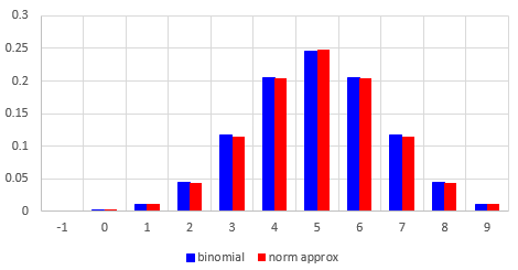
To finish off, let’s look briefly at how the binomial distribution and its normal approximation compare in this inappropriate case. First, if we had p = 0.5 as in the usual pictures we see (like the one I showed from Wikipedia above), the approximation would be quite close (note that np and nq are both 5), as shown in this side-by-side bar graph:
Here is a rough picture of the normal distribution itself superimposed on the binomial:
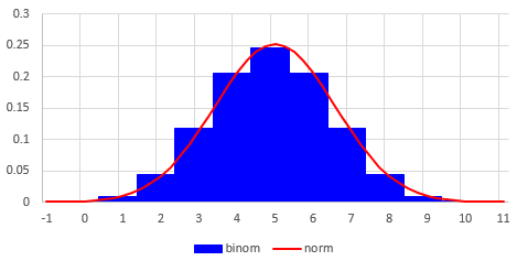
(The normal is shifted a little to the right, because of how I made this in Excel.)
But for our actual problem, here is how the approximation fares:
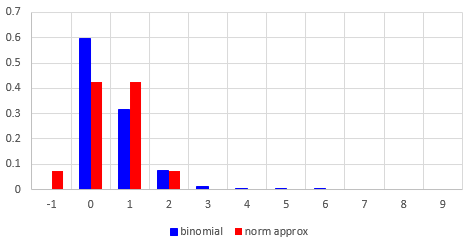
As we found, the probability that x is greater than 0 is 0.5, according to the approximation, but it’s only 0.4 in reality. Here are the binomial and normal superimposed:
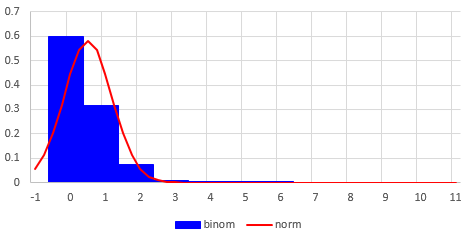
They don’t look alike at all. Clearly, the instructions to use the approximation were not a good recommendation – except if you want to learn why you shouldn’t do it!