Last time we introduced standard deviation. Here we’ll look into why two formulas (namely, population and sample standard deviation) are different, and why several different formulas for either are equivalent. We’ll also discover how to update the standard deviation when a new value is added. In doing so, we’ll see some different perspectives than we find in a textbook.
Population vs sample standard deviation
A 2001 question brings up an important distinction that we largely ignored last time:
Sample and Population Standard Deviation

What letters represent theoretical and 'real' standard deviation, mean, and variance?
The mention of different “letters” implies that Lara is asking about symbols like “s” and “σ“, using nonstandard words for an important distinction.
Doctor Jordi answered, going beyond the distinction of symbols to talk about their meanings:
Hello, Lara - thanks for writing to Dr. Math.

"Theoretical" and "real" standard deviation?  I am not very sure what you mean, but I am guessing that you are talking about *sample* standard deviation and *population* standard deviation.
Perhaps Lara’s wording comes from seeing the sample as taken from a theoretical probability distribution (rather than from a specific population), making the sample the only real data involved. That’s how Doctor Jordi will be seeing it.
The traditional symbol for the sample standard deviation is S (lowercase or uppercase; there is a slight difference between the two) and the equivalent Greek letter sigma (which looks like an o with a little tail sticking out from the top) is commonly used to denote the population standard deviation. Also recall that S^2 is called the sample variance and sigma^2 is called the population variance; these two are probably the ones you will work with the most.
We have these notations:
- \(\bar{x}\) (“x-bar”): sample mean
- \(\mu\) (Greek “mu”): population mean
and then
- \(s\): sample standard deviation
- \(\sigma\) (Greek “sigma”): population standard deviation
- \(s^2\): sample variance
- \(\sigma^2\) (Greek “sigma squared”): population variance
Since the Greek letter sigma (σ) represents our “s“, these derive from the word “standard”. (That’s a little odd because the main idea is not that it is “standardized”, but that it represents a “deviation”. But we use “d” and “δ” for too many things already!)
The capital S is used when treating it as a random variable in itself.
First, for a sample:
Formally speaking, their mathematical definitions are as follows.

     S^2 = Sum(i=1 to n)(X_i - Xbar)^2
           ---------------------------
                     n - 1

Where X_i denotes the i th value in our sample, the i th realization of the random variable X, and Xbar, written as a X with a bar above it, denotes the sample mean (again, not to be confused with the population mean).
That is, $$s^2=\frac{\sum_{i=1}^n\left(x_i-\bar{x}\right)^2}{n-1}$$
The standard deviation is the square root of this. Note that this formula expresses just what we saw last time, except that, as briefly mentioned then, we use \(n-1\) in the denominator, rather than \(n\), when we are using the standard deviation of a sample not just to describe the sample itself, but to estimate the standard deviation of the population from which the sample came. More on that to come, with fuller explanations next time.
What about a population? He expresses this in terms of a random variable with a known probability distribution, rather than a literal population (in the sense of a collection of individuals, from which a sample is drawn), which is how many readers will expect to see it:
     sigma^2 = E((X - mu)^2)

Where E denotes the expected value function, which you may or may not have encountered already. Roughly, the expected value function tells you the value "on average" that we would expect the expression sent as input to the function to take. For example, the expected value of the random variable X, E(X), would be the value we expect this variable to take on average, which is nothing more than the population mean. In fact, mu is defined to be E(X).
That is, we define the standard deviation of a probability distribution as $$\sigma^2=\mathrm{E}\left(\left(x-\mu\right)^2\right),$$ where \(\mu\) is the mean of the distribution.
Since the expected value is just the average (mean), when we are talking about a population of individual values \(x_i\). this is the same as $$\sigma^2=\frac{\sum_{i=1}^n\left(x_i-\mu\right)^2}{n}.$$
There is a distinction here that I don’t generally see in introductory statistics. There, we think of a population as merely a set of values (such as the heights of everyone in a country). But ultimately, we think of a population as representing all possible people, and the distribution as a process by which those people are generated. (For example, when we say that a physical population is normally distributed, we aren’t saying that the actual values in the population exactly follow the normal distribution – which is continuous, not discrete! – but that we assume that the population is generated by a process that follows the normal distribution. So even the population is really a large “sample” from such a process.)
This is how Doctor Jordi will view it in his example.
Sample vs population: a measurement example
Be careful of the distinction of the population and sample variances (or standard deviations), as they have different definitions. You have to realize the difference between a sample and the population it was drawn from. For example, say you are using a thermometer to measure the freezing point of water. Say that this thermometer can measure very small changes in temperature, but that it does not always measure the same temperature in the same way; it can be a little off to one side or to the other. Say you have taken five measurements of the freezing point of water with this thermometer, which were the following (in Fahrenheit):

     32.1 32.3 32.6 31.8 31.8

In this setup, the sample is our five numbers above, and the population is the abstract infinity of all possible values our thermometer can display for the freezing point of water. You can take the average of these five values in our sample, which we will now call the sample mean instead of average, and you will find that it is Xbar = 32.12 (just add all values and divide by 5).
Note that here, “population” is not a literal collection of many individuals (as it is, for example, when the sample is a survey of people), but the theoretical behavior of the thermometer: all possible values it could display for this measurement.
The sample mean here is $$\frac{\sum x_i}{n}=\frac{32.1+32.3+32.6+31.8+31.8}{5}=\frac{160.6}{5}=32.12$$
(I’ve changed one number and the resulting calculations, because there was an error in the original.)
Now, we know that the freezing point of water should be 32 degrees Fahrenheit; in fact, our thermometer was probably calibrated to read 32 degrees for freezing water, so can we conclude from our experiment that the freezing point of water is not 32 degrees? No, because our sample mean need not be equal to the population mean. The population mean is mu = 32 degrees.  In fact, if we were to take many, many, more readings (say, 1000) would you expect our sample mean (the average of the readings) to get closer to or farther away from 32, the population mean?

The assertion that we expect the sample mean to get closer and closer to the population mean as the sample size gets larger and larger is called the Law of Large Numbers. It is a very intuitively pleasing statement, and it can be proven using a few assumptions from probability theory, but I will not go into that right now.
We discussed the Law of Large Numbers here.
Let's go back to our sample of thermometer readings.  What is the sample variance, S^2?  Just by using the definition of S^2, we find that

     S^2 = (32.1 - 32.12)^2 + (32.3 - 32.12)^2 +
           (32.6 - 32.12)^2 + (31.8 - 32.12)^2 +
           (31.8 - 32.12)^2
           -------------------------------------
                          5 - 1

  so S^2 = 0.117        <------------------ sample variance

     S   = 0.34205 (approximately) <------ sample standard deviation
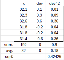
In detail: $$s^2=\frac{\sum_{i=1}^n\left(x_i-\bar{x}\right)^2}{n-1}\\=\frac{(32.1-32.12)^2+(32.3-32.12)^2+(32.6-32.12)^2+(31.8-32.12)^2+(31.8-32.12)^2}{5-1}\\=\frac{(0.02)^2+(0.18)^2+(0.48)^2+(-0.32)^2+(-0.32)^2}{4}\\=\frac{0.0004+0.0324+0.2304+0.1024+0.1024}{4}=\frac{0.468}{4}=0.117$$
$$s=\sqrt{0.117}\approx0.342$$
This can be calculated using a simple table:
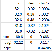
(In the “avg” row, we divided the sum of x by n, and the sum of squared deviations by \(n-1\).)
This tells us something about the accuracy of our thermometer. The sample standard deviation roughly says that on average, our thermometer will be about 0.34 off from the 'true' value. That could be a large or small standard deviation, depending on what we want the uses of this thermometer to be. However, the sample standard deviation that we have calculated here is subject to change. If we repeat this experiment and take five more values, we are likely to get a different variance. If we take five thousand readings, we are again likely to get a slightly different variance, but close to a certain value. If we were to take five million readings, our sample variance would get closer to a certain value. In short, the more readings we take, the closer our sample variance (or sample standard deviation) should be to the population variance (or population standard deviation). That is, we can use S^2 to estimate sigma^2, and the goodness of the estimation of sigma^2 using S^2 should be better if we increase the sample size. We say that S^2 is a consistent estimator of sigma^2.
Theoretical calculations show that in order for the sample variance to accurately estimate the population variance, we need that \(n-1\) rather than just \(n\) in the denominator. We’ll see more about that next week, though even then we won’t try to show all the details.
Sometimes it is possible in advance to know the population variance if we know the population mean and the distribution of the random variable in question (our random variable in our thermometer example was the reading of the thermometer). Most often, in real life, we know neither of these two, so we can use the sample mean and variances to make estimates about them.

In fact, that's what statistics is all about: making inferences about unknown populations using data collected from samples. Always keep that in mind as you pursue your studies in statistics.
And that is the (very basic) idea behind the difference in the formulas for sample and population standard deviation.
But you’ll see different formulas in a very different sense, as well.
A second formula for the same thing
From 2007, we have a question about this other difference in formulas:
Are Two Formulas for Finding Standard Deviation the Same?

My statistics text states that a shortcut formula for calculating sample standard deviation is to take the square root of [(the sum of x^2) minus (the sum of x)^2/n all divided by n-1].  Is this really a shortcut formula for calculating S.D.?

I am confused to how this equation is equal to the standard deviation formula that I was initially taught, which is the square root of [the sum of (x minus x bar)^2 divided by n-1].  Can you explain how these formulas are equal to one another?

I have been trying to factor the original equation [i.e. (x-x bar)(x-x bar), but multiplying that out still does not seem to show a way to obtain the shortcut method from the original formula.
That is, whereas the definitional formula for standard deviation is $$s=\sqrt{\frac{\sum_{i=1}^n\left(x_i-\bar{x}\right)^2}{n-1}},$$ this alternative formula is $$s=\sqrt{\frac{\sum_{i=1}^n x_i^2-\frac{1}{n}\left(\sum_{i=1}^n x_i\right)^2}{n-1}}$$
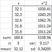
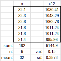
It is easier to calculate, especially when the data are integers but the mean is not, so that the deviations are hard to calculate. To demonstrate, let’s use the alternative formula for our sample temperatures above, 32.1, 32.3, 32.6, 31.8, 31.8. We get $$s=\sqrt{\frac{\sum x^2-\frac{1}{n}\left(\sum x\right)^2}{n-1}}\\=\sqrt{\frac{\left(32.1^2+32.3^2+32.6^2+31.8^2+31.8^2\right)-\frac{1}{5}\left(32.1+32.3+32.6+31.8+31.8\right)^2}{4}}\\=\sqrt{\frac{\left(1030.41+1043.29+1062.8+1011.24+1011.24\right)-\frac{1}{5}\left(32.1+32.3+32.6+31.8+31.8\right)^2}{4}}\\=\sqrt{\frac{5158.94-5158.472}{4}}=\sqrt{\frac{0.468}{4}}=\sqrt{0.117}\approx0.342$$ just as before.
We can evaluate this using an even simpler table:
I answered:
Hi, Ashley.

This is hard to type, so I'll use "m" for "x bar", and a few other notations that I hope will be clear:

Definition:

  sqrt(SUM[(x - m)^2] / (n-1))

where

  m = SUM[x] / n

Desired formula:

  sqrt( (SUM[x^2] - (SUM[x]^2)/n) / (n-1) )
That is, the definitions are
$$\bar{x}=\frac{\sum x}{n}$$
$$s=\sqrt{\frac{\sum\left(x-\bar{x}\right)^2}{n-1}},$$
and the new formula is $$s=\sqrt{\frac{\sum x^2-\frac{1}{n}\left(\sum x\right)^2}{n-1}}.$$
Now let's do what you started to do, and see if we can manipulate the definition to look like the shortcut:

  Std Dev = sqrt(SUM[(x - m)^2] / (n-1))

          = sqrt(SUM[(x - m)(x - m)] / (n-1))

          = sqrt(SUM[x^2 - 2mx + m^2] / (n-1))

          = sqrt((SUM[x^2] - SUM[2mx] + SUM[m^2]) / (n-1))

          = sqrt((SUM[x^2] - 2m * SUM[x] + n * m^2) / (n-1))

Are you okay so far?  The next to last step rearranges the sum.  The last factors the constant 2m out of the second sum, and rewrites the third sum, which was the sum of n copies of a constant, m^2, making a total of n * m^2.
That is, $$s=\sqrt{\frac{\sum\left(x-\bar{x}\right)^2}{n-1}}\\=\sqrt{\frac{\sum\left(x-\bar{x}\right)\left(x-\bar{x}\right)}{n-1}}\\=\sqrt{\frac{\sum\left(x^2-2\bar{x}x+\bar{x}^2\right)}{n-1}}\\=\sqrt{\frac{\sum\left(x^2\right)-\sum\left(2\bar{x}x\right)+\sum\left(\bar{x}^2\right)}{n-1}}\\=\sqrt{\frac{\sum x^2-2\bar{x}\sum x+n\bar{x}^2}{n-1}}.$$
Now let's use the definition of x bar (my m):

  = sqrt((SUM[x^2] - 2 SUM[x]/n * SUM[x] + n * (SUM[x]/n)^2) / (n-1))

  = sqrt((SUM[x^2] - 2 SUM[x]^2 / n + SUM[x]^2 / n) / (n-1))

  = sqrt((SUM[x^2] - SUM[x]^2 / n) / (n-1))

There you have it!
Again, $$\sqrt{\frac{\sum x^2-2\bar{x}\sum x+n\bar{x}^2}{n-1}}\\=\sqrt{\frac{\sum x^2-2\frac{\sum x}{n}\sum x+n\left(\frac{\sum x}{n}\right)^2}{n-1}}\\=\sqrt{\frac{\sum x^2-2\frac{\left(\sum x\right)^2}{n}+\frac{\left(\sum x\right)^2}{n}}{n-1}}\\=\sqrt{\frac{\sum x^2-\frac{\left(\sum x\right)^2}{n}}{n-1}}$$
Multiplying numerator and denominator by n, we can also rewrite this as $$s=\sqrt{\frac{n\sum x^2-\left(\sum x\right)^2}{n(n-1)}}$$
If you already calculated the mean, you can simplify this to $$s=\sqrt{\frac{\sum x^2-n\left(\bar{x}\right)^2}{n-1}}.$$
And for a population, it becomes $$\sigma=\sqrt{\frac{n\sum x^2-\left(\sum x\right)^2}{n^2}}=\sqrt{\frac{\sum x^2}{n}-\bar{x}^2}.$$
Ashley replied:
Dr. Peterson-

Thanks for your help!  I had been working on that for hours, but I guess I just needed to do a few more steps of factoring out.  I really appreciate it!  :)

~Ashley
We can do essentially the same thing to convert the definition we saw above for the standard deviation of a probability distribution into a form that was mentioned in passing last time: $$\sigma^2=\mathrm{E}\left(\left(x-\mu\right)^2\right)=\mathrm{E}\left(x^2-2x\mu+\mu^2\right)\\=\mathrm{E}\left(x^2\right)-\mathrm{E}\left(2x\mu\right)+\mathrm{E}\left(\mu^2\right)=\mathrm{E}\left(x^2\right)-2\mu\mathrm{E}\left(x\right)+\mu^2\\=\mathrm{E}\left(x^2\right)-2\mu^2+\mu^2=\mathrm{E}\left(x^2\right)-\mu^2\\=\mathrm{E}\left(x^2\right)-\left(\mathrm{E}\left(x\right)\right)^2$$ which is exactly the last expression above.
Recalculating with new data
The alternate formula helps answer this question from 2002:
Re-Calculating the Standard Deviation

How can I re-calculate the standard deviation of a set of values when I insert a new value but I don't know what the existing values are?

For instance, I have a set of 5 values. They have an average of 20 with a standard deviation of 12. If I add the value 26 to the set I can re-calculate the new average of 21, but how do I re-calculate the new standard deviation?
This would be very hard to do using the original formula (the definition). But with the alternative formula, it is not bad at all!
Doctor TWE answered:
Hi Gareth - thanks for writing to Dr. Math.

Yes, this can be done.

If you are working with population mean and standard deviation, an alternate formula for the population standard deviation (the one calculators and computers actually use) is

             n*Sum[x^2] - (Sum[x])^2
   s = Sqrt[ ----------------------- ]
                       n^2

where

   n        = the population size (number of data points)
   Sum[x^2] = the sum of the squares of all data points
   Sum[x]   = the sum of all data points

So if you could recover the values of Sum[x^2] and Sum[x], then the standard deviation after adding a new value, v, would be

              (n+1)*(v^2 + Sum[x^2]) - (v + Sum[x])^2
   s' = Sqrt[ --------------------------------------- ]
                             (n+1)^2
The formula he starts with is the form we showed above for a population, $$\sigma=\sqrt{\frac{n\sum x^2-\left(\sum x\right)^2}{n^2}}$$ and the last formula is $$\sigma’=\sqrt{\frac{(n+1)\left(v^2+\sum x^2\right)-\left(v+\sum x\right)^2}{(n+1)^2}},$$ using \(n+1\) because there is now one more data point.
Recovering Sum[x] is easy: it's just n times the mean, mu:

   Sum[x] = n*mu

Recovering Sum[x^2] is a little trickier.  Starting from the formula,

                                n*Sum[x^2] - (Sum[x])^2
                      s = Sqrt[ ----------------------- ]
                                          n^2

                           n*Sum[x^2] - (Sum[x])^2
                    s^2 =  -----------------------
                                     n^2

                n^2 s^2 =  n*Sum[x^2] - (Sum[x])^2

   n^2 s^2 + (Sum[x])^2 = n*Sum[x^2]

     n^2 s^2 + (n*mu)^2 = n*Sum[x^2]

     n^2 s^2 + n^2 mu^2 = n*Sum[x^2]

        n^2(s^2 + mu^2) = n*Sum[x^2]

          n(s^2 + mu^2) = Sum[x^2]

So from n, mu, and s, we can recover Sum[x] and Sum[x^2], which means we can compute s'.
So we have $$\sum x=n\mu\\\sum x^2=n\left(\sigma^2+\mu^2\right),$$ and if we insert these in the formula we obtained before, we get $$\sigma’=\sqrt{\frac{(n+1)\left(v^2+n\left(\sigma^2+\mu^2\right)\right)-\left(v+n\mu\right)^2}{(n+1)^2}}\\=\sqrt{\frac{n\left((v-\mu)^2+(n+1)\sigma^2\right)}{(n+1)^2}}$$
Let’s check this, using the example from above (but as a population), we have \(n=5\), \(\mu=32.12\), and \(\sigma^2=0.0936\):
Adding a sixth value, 31.4, we find that the new population standard deviation is $$\sigma’=\sqrt{\frac{n\left((v-\mu)^2+(n+1)\sigma^2\right)}{(n+1)^2}}=\sqrt{\frac{5\left((31.4-32.12)^2+(5+1)0.0936\right)}{(5+1)^2}}\\=\sqrt{\frac{5\left((-0.72)^2+6(0.0936)\right)}{6^2}}=\sqrt{\frac{5(0.5184+0.5616)}{36}}=\sqrt{0.15}=0.3873$$
That’s just what we get using the alternative formula with all the data:
Repeating that for a sample
A similar computation can be made if you have a sample mean and standard deviation. The alternate formula for the sample standard deviation is:

               n*Sum[x^2]-(Sum[x])^2
     s = Sqrt[ --------------------- ]
                      n*(n-1)

So you start from there, but the rest is the same.
This time we solve to get $$\sum x=n\bar{x}\\\sum x^2=(n-1)s^2+n\bar{x}^2,$$ which we insert into $$s’=\sqrt{\frac{(n+1)\left(v^2+\sum x^2\right)-\left(v+\sum x\right)^2}{n(n+1)}}$$ to obtain $$s’=\sqrt{\frac{(n+1)\left(v^2+(n-1)s^2+n\bar{x}^2\right)-\left(v+n\bar{x}\right)^2}{n(n+1)}}\\=\sqrt{\frac{\left(nv^2+n(n-1)s^2+n^2\bar{x}^2\right)+\left(v^2+(n-1)s^2+n\bar{x}^2\right)-\left(v^2+2nv\bar{x}+n^2\bar{x}^2\right)}{n(n+1)}}\\=\sqrt{\frac{n\left(v-\bar{x}\right)^2+(n^2-1)s^2}{n(n+1)}}$$
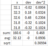
Let’s check this. For the original 5 values, as a sample, the mean was \(\bar{x}=32.12\), and the sample variance was \(s^2=0.117\). When we add the sixth data point of 31.4, we get a mean of 32 and a variance of 0.42426 (here calculated both ways):
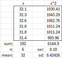
Our formula gives $$\sqrt{\frac{n\left(v-\bar{x}\right)^2+(n^2-1)s^2}{n(n+1)}}=\sqrt{\frac{5\left(31.4-32.12\right)^2+(5^2-1)0.117}{5(5+1)}}\\=\sqrt{\frac{5\left(0.5184\right)+24(0.117)}{30}}\approx \sqrt{0.18}=0.42426$$
So it’s correct.
Pingback: Sample Standard Deviation as an Unbiased Estimator – The Math Doctors